It is said that OpenAI may very possibly have constructed a counterexample to the Hodge conjecture.André Weil was one of the earliest mathematicians to doubt the Hodge conjecture and to attempt to construct counterexamples, and perhaps also one of those who came closest to doing so successfully.
Weil actually had little direct interaction with Hodge himself. The earliest record seems to be from 1947, when Weil mentioned in a letter to H. Cartan that he was studying Hodge’s book and trying to apply it to algebraic varieties.
Weil strongly recognized the importance of Hodge theory, but at the same time sharply criticized its notation as looking like “a horrible salad of tensors.”
Ten years later, Weil wrote Introduction à l’étude des variétés kählériennes, rewriting and organizing the Kähler–Hodge techniques in a cleaner language, while stating that this was done to “facilitate the reader’s understanding.”
The notation and organization of Hodge theory in its modern form were to a large extent fixed in Weil’s book. Following Weil’s passing, the book was singled out in his obituary as the first modern exposition of Hodge theory.
Then came the famous first postwar Fields Medal. Hodge was among the members of the committee who most strongly supported awarding it to Weil, warning that otherwise they “might be shirking our duty.” His efforts ultimately did not prevail. Perhaps to spare future committees from facing quite the same dilemma, the Fields Medal would later acquire its famous age limit of forty.
At the International Congress of Mathematicians where the prizes were awarded, Weil gave a plenary lecture presenting a unified perspective on number theory and algebraic geometry, summarizing and anticipating much of the development of algebraic geometry over the following decades. Five days later, Hodge presented the original version of the Hodge conjecture in another lecture.
The early Hodge conjecture looked like a natural extrapolation of Lefschetz’s (1,1)-theorem, so there were not many reasons to doubt it.
Lefschetz had already solved the case (p=1), and degree-2 Hodge classes all come from divisors. Therefore, if the entire Hodge ring of a variety were generated by degree-2 Hodge classes, the Hodge conjecture would follow automatically.
In the 1960s, Mumford and Tate tried precisely to pursue this route. Unfortunately, Mumford found a counterexample that cut off this approach, namely the so-called exceptional Hodge classes. The example is a CM-type abelian fourfold (A) possessing Hodge ((2,2)) classes that cannot be written as products of divisors.
What happened next is known from a letter Tate wrote to Serre.
In 1965, Tate told Weil about this counterexample. Weil quickly realized that this example was essentially only a special case of a 4-dimensional family of examples.
He then considered a class of special abelian varieties with an additional imaginary quadratic field symmetry. This symmetry divides the complex directions evenly into two groups. Taking the product of these directions over the imaginary quadratic field gives a two-dimensional rational cohomology subspace. The fact that the two groups have equal size ensures that this space is of ((n,n))-type, and therefore it is a two-dimensional Hodge class space: what later became known as the Weil classes.
These Weil classes arise automatically from symmetry and linear-algebraic structure, without any need to know in advance of a corresponding algebraic subvariety. Weil therefore began to doubt the conjecture: if these classes can be generated automatically in this way by symmetry, why must they necessarily correspond to genuine algebraic cycles? If even one Weil class could be shown not to correspond to any algebraic cycle, the Hodge conjecture would be disproved. In this way, a counterexample to one possible proof strategy was generalized by Weil into a possible counterexample to the conjecture itself.
As you and Mumford seem to believe Hodge’s conjecture, it is now up to you to exhibit algebraic cycles corresponding to these abnormal classes. As I incline to disbelieve it, I shall rather attempt to show that there is no such cycle.
Weil then began trying to construct a counterexample. Of course, his efforts did not succeed; otherwise the conjecture would not later have become one of the Millennium Prize Problems.
This was much like Weil’s work on the Mordell/Riemann conjectures, and even on the Fermat and Langlands conjectures. Faced with these great conjectures, he could either make an initial breakthrough that no one had achieved for a century, or immediately recognize the importance of a conjecture, or of a particular route toward its solution, for the future development of mathematics, and thereby help direct the course of the subject as a whole. Although in the end he was usually not the final solver of these problems, Weil may be precisely the kind of mathematician most needed in the AI era.
Later still, according to Benedict Gross’s recollection, at a conference celebrating Ahlfors’s seventieth birthday about ten years later, Weil was still publicly discussing, in a rather provocative way, how one might attack the Hodge conjecture.
Gross, who was still at an early stage of his career, sat in the audience trying to modify Weil’s ideas in order to prove a period identity related to the Chowla–Selberg formula, and soon turned the argument into a paper.
At the same conference, Serre introduced him to Deligne, and Gross then explained this result obtained by adapting Weil’s ideas.
Deligne was astonished and asked Gross: “Have you proved the Hodge conjecture?”
Gross cheerfully replied that if that were really the case, he would certainly be pleased. He was still looking for a PhD thesis topic, and proving the Hodge conjecture should presumably be enough for a thesis.
A few weeks later, Deligne sent Gross a three-page manuscript. That manuscript eventually developed into the famous result that all Hodge cycles on abelian varieties are absolutely Hodge.
When Milne discussed this history, he remarked that in relation to Weil’s doubts, abelian varieties should originally have counted as one of the easier cases of the Hodge conjecture.
Yet after fifty years, the mathematical community still could not prove that these Weil Hodge classes are algebraic. This obviously did a great deal to weaken mathematicians’ confidence in the Hodge conjecture……
As for what came later in the history of the Hodge conjecture—Grothendieck, Deligne, Griffiths, and the rest—that will have to be added another time.
Finally, regarding the possibility that OpenAI may have constructed a counterexample to the Hodge conjecture, Weil’s own words may be especially appropriate:
“La question que pose la “conjecture de Hodge” est bien naturelle… Par malheur, en d´epit du mot de “conjecture”, il n’y a, que je sache, pas l’ombre d’une raison d’y croire; on rendrait service aux g´eom`etres si l’on pouvait trancher la question au moyen d’un contre-exemple.”
“The question posed by the ‘Hodge conjecture’ is a very natural one… Unfortunately, despite the word ‘conjecture’, as far as I know there is not the slightest reason to believe it; one would be doing geometers a service if the question could be settled by means of a counterexample.”
Last year, I repaired an NZXT Signal 4K30 USB capture device that I bought on eBay for cheap. It was completely dead, and the cause turned out to be a bad solder joint on an inductor, which prevented power from getting to a crucial part of the board.
After I fixed it, I tried using it to capture signals from a bunch of different HDMI source devices to make sure it worked correctly. As I said in my last post about it:
I did find one 720p60 HDMI source that it doesn’t like — the captured video shows up as pink and green.
In that post, I also pointed to a few Reddit threads (1, 2) where similar issues had been observed on a PS5 and Nintendo Switch, respectively.
Here’s a snapshot of what captured video looked like from the one HDMI source that it didn’t like:
You can see that the colors are green and purple. They’re completely wrong. I knew from past experience with video encoders and decoders that this is very typical behavior if you have a mismatch between RGB and YUV video. I doubted it was faulty hardware, especially since other people on Reddit had seen the exact same symptom.
I left it at that. I didn’t care that this one device wouldn’t capture correctly, and I didn’t bother contacting NZXT about it. I’ve noticed that since then, the device seems to have completely disappeared from the market. You can’t buy it on Amazon or Newegg anymore, and NZXT’s website doesn’t mention it anywhere except under support. It’s pretty clear that NZXT exited the capture card market. If I contacted them now, I’d be shocked if they could do anything about it.
Last night, a thought randomly jumped into my mind. I’ve been using Claude to do some pretty in-depth reverse engineering and bug investigations lately. For example, here’s a reverse-engineered Linux kernel V4L2 driver for the Elgato Game Capture HD60 S that I investigated in depth a couple of years ago. What if I had it look into this problem? It would be a nice way to completely finish off the first post where I repaired the hardware problem. Together, could we fix the final issue, which I assumed was a firmware problem?
During the hardware repair, I had already documented all of the different components used in the device, so I gave that all to Claude, along with a description of the problem, pictures of the issue from the Reddit posts, NZXT’s last firmware update for the device released in 2022, and a checkout of a GitHub repository containing ITE’s driver for the IT6805 HDMI receiver IC used by the Signal 4K30. I also pointed out that I suspected it was some kind of RGB vs. YUV mismatch because I’ve seen this happen in the past when developing firmware for video devices.
15 minutes or so later, Claude got back to me with results. It agreed that it was a YUV vs. RGB mismatch issue. It pointed out what it thought were a few bugs in the firmware that looked promising. To be sure, it asked me to verify a few things about the detected signal. It told me that the Cortex-M0 microcontroller has a UART with debug output. I found the unmarked debug header on the PCB, figured out which pin was the TX pin (and the baud rate) with my portable oscilloscope, captured its output with the problematic HDMI source device attached, and pasted it back. I also used my reverse-engineered Game Capture HD60 S Linux driver listed above to provide more details about what type of signal the problematic source was outputting.
The source device was outputting in DVI mode instead of HDMI mode. This was a major clue. DVI mode means it doesn’t have some of the extra packets that are included with newer HDMI sources, such as AVI InfoFrames.
Claude pinpointed a section of code in ITE’s stock IT6805 driver that looked wrong, and confirmed this code was also present in NZXT’s firmware. Here’s a trimmed-down snippet:
This code is figuring out whether the IT6805 has detected an HDMI or DVI signal, and configuring various registers based on that result. One such register tells the IT6805 how to decode the incoming video signal. If it’s an HDMI signal, it grabs the color mode directly from the AVI InfoFrame and puts it into bits 4 and 5 of register 0x6B.
On the other hand, if it’s a DVI signal, it knows that the video signal has to be RGB, so it tries to configure those same bits in register 0x6B for RGB mode.
Except…the code is wrong. The comment correctly says it should be configured for RGB in this case (“seting input format to RGB”) but what it actually does is write 01 to bits 5:4, which means YUV 4:2:2 mode according to the comment at the top.
I can’t speak for certain, but I think I see the mistake the original ITE developer made. When my eyes first jump to the comment for RGB mode, what sticks out in my mind is “RGB mode – 01”. But that’s my brain parsing the comment incorrectly. What it really says is “00: RGB mode”. I think the fact that the comment only uses that one hyphen and then uses commas for everything else throws me off. I wouldn’t be surprised if the original developer made the same kind of parsing error in their brain.
Okay, so I now had a theory. How could I test it? The debug UART unfortunately didn’t provide a way to read or write the IT6805’s registers, or I could have easily tested it out.
In exchange for a fun story and the potential to be able to release this fix for everyone, I was willing to risk bricking my device. Claude was very hesitant about this and wanted me to try accessing the MCU through SWD to back up its firmware first, but I decided to just full send it. I’ll bet the chip was locked anyway. I had Claude reverse engineer the NZXT firmware updater utility to figure out how it works, and also figure out if it would be safe to simply patch the firmware to change it to write 00 rather than 01 to those bits in register 0x6B. I was particularly worried about changing a checksum or CRC in the firmware image, but Claude was pretty sure the MCU firmware was not checksummed in any way. It fixed the bug in ITE’s driver by patching a single byte in the NZXT firmware to change a movs r2, #16 instruction to movs r2, #0.
Claude also gave me back a command-line utility that reflashes the firmware using the DLL included with NZXT’s updater. I couldn’t just use NZXT’s stock utility because it refuses to install a firmware update file if it thinks the device is already up to date.
Despite the potential that I could render my capture card completely inoperable, I decided to run the updater. It went through the whole update process, which ended looking like this:
I power cycled the capture card as the instructions told me to, and then opened up OBS to see if the behavior changed at all.
To my relief, it all still worked after the update, and even better, the bug was gone! The colors looked perfect when capturing my DVI source device.
That was definitely the bug. It’s actually a bug in ITE’s driver, so it probably affects lots of devices that just drop in this vendor code without actually testing it against a bunch of different HDMI sources and sinks.
In my case, the source device I’m using doesn’t provide InfoFrames at all, so an HDMI sink device encountering a signal without InfoFrames is supposed to assume the data is RGB. As for other people’s situations, they could hit this same problem even with a modern HDMI source device if they have an old DVI monitor attached to the passthrough port whose EDID doesn’t support HDMI mode for whatever reason.
It’s very possible that the PS5 and Switch in the Reddit posts were encountering a completely different problem that happened to have the same symptom. All I know is Claude’s bug fix actually worked for me, and now I can use this capture card to capture this particular sink device with perfect, vibrant colors!
In case it is useful for someone else in the future with the same discontinued NZXT Signal 4K30 capture card, I’m providing the firmware bug fix to the community. Here’s my GitHub repository for it, along with installation instructions: https://github.com/dougg3/nzxt-signal-4k30-color-bug-firmware-patch/
My mind is still pretty blown away by how good Claude has become at hunting for bugs and reverse engineering firmware. I didn’t run into any problems during this particular analysis, but I will say that sometimes I run into Claude’s cybersecurity guardrails when trying to track down issues. I understand why these safeguards are in place, but it can be frustrating at times. I’m not officially a cybersecurity professional, so I’m not sure if it would be worth even trying to apply to their Cyber Verification Program. But I think there are times when reverse engineering and even local hardware-in-hand exploits have legitimate non-nefarious purposes, like being able to replace a sketchy device’s buggy closed firmware with an alternative, improved open-source firmware. I wish there was a way as a hobbyist to communicate that intent to Anthropic without being hit with the guardrails!
Anyway, I didn’t run into that problem at all on this project. I would say that overall, this fix was a complete success! I tested it out with several HDMI source devices after patching the firmware, and now they all work great. It feels great to fully close the book on my Signal 4K30 repair story.
By the way, the sample picture I used for showing the color problem came from the Kodak Lossless True Color Image Suite. And yes, it was a direct capture from the 4K30 before and after the firmware fix!
An experiment to design a cute PCB (without touching any tools) in plain English
hardwarepcbkicadaiclaude 8 min
The board I will be journaling about.
I have been wanting to design a simple PCB for the last couple of years now. The thought of converting a design idea into a physical board and programming it to do things is fascinating to me. Long story short, I procrastinated until I tried to vibe-generate a dead simple PCB with Claude Opus 4.8 and it was terrible ! It had no idea about the orientation of the components, it did not do any proper routing. I was disappointed and accepted the fact that these tools were not there yet.
Then arrived the Fable 5. At first I was not that hopeful. One Thursday evening, around 10 hours before my weekly reset for Claude, I decided to give it another try; this time with Fable 5.
I had two rules:
No manual edits or verification of the board.
Every problem I face before manufacturing will be solved by Fable.
This meant I was going to trust Fable with my wallet. I decided to describe the board I want it to generate, and I was not going to be involved in the design phase. I was the end customer.
This is the prompt I gave it:
That was it, a short description of a RPI 2350 based development board which can drive an E-ink display. After working autonomously for a couple of hours it came up with the design shown in the video below.
<!– YOUTUBE: when the video is up, replace this
Everything else in this figure — the frame, the caption — stays. –>
The board as it freshly came out of Kicad ⃰.
Board
31.8 × 37.32 mm, 4 layer
MCU
RP2350A
Display
1.54″ E-ink, 200×200
Flash
8 MB QSPI
Cost
26€ per board
A closer look to some errors
The design process was not error free of course. When I showed the initial design (Claude was still working on it) of the PCB to my colleague, the first thing he wanted me to check (after recovering from the pain of seeing them tracks) was the DRC (Design Rule Checking) errors. I did not know what it was, and when we looked at it, there were indeed 65 DRC errors. Following the rule, I only mentioned the errors to Fable and did nothing else.
Front: Beautiful placement, with two mistakesBack: horrendous tracks
Fable was amazing at component selection, except for the two components I highlighted above. The big one on the top left is the SPI flash which stores the firmware and other data that you want to save. The SPI flash memory Claude chose was W25Q128JVS. It comes with the SOIC-8 wide package, but the pads designed for the memory was for a SOP-8 package, meaning the chip is too big for the pads. The bottom left component on the other hand is the transistor that switches the boost converter for the E-ink driver circuitry. As you can see it also chose the wrong package, as it is too small for the pads. I did not realise these until I uploaded the required files to JLCPCB. There I could see the issues, and I discussed it with Claude. For the W25Q128JVS it insisted that there was a SOP-8 package but I could not find it in LCSC’s library. Eventually we settled at the P25Q64SH chip.
But wait a minute, how did it even route ?
The design had 65 footprints, 54 nets and 118 unconnected lines. It is not a complex PCB by any means :P. Fable decided to use the Freerouting open-source project. The tool worked for 2 minutes, and after seventeen passes it plateaued at sixty nine connections, leaving 49 disconnected, and it could not finish the job. The remaining connections were hand-routed by Claude.
Freerouting doing its job
After I ordered the board my colleague mentioned to me the KiCadRoutingTools open-source project. It ran for 1.25 seconds and it could route all the connections with no problem. I will try this tool out for my upcoming hardware projects.
Same placement, two routers
Ordering with JLCPCB
I had never ordered anything from a PCB manufacturer before. It seemed complex and I was reluctant to take the first step. Upon Claude’s compilation of the project, I asked it to prepare the required files for JLCPCB, and tell me what to select on their GUI. Man am I satisfied with JLCPCB. It was so straight forward, easy to interact with and there was no bloat. I uploaded the files, some components Claude selected were not available, we did a back and forth and voila we were done. For five fully assembled boards I paid 130 Euros, ordered the E-ink displays from a local shop and now it was the waiting game.
Some cool animations while we are waiting for the PCBs
The four layers, pulled apart.Assembly of our board
The boards have arrived !!!
I received the PCBs and the first thing I wanted to do was to plug it in to my laptop. I have broken multiple USB modules for my Framework earlier, hence I thought checking for a short between 3v3 and ground was a no-brainer, although my colleague was suggesting me to just yeet it since this was a fully vibe-generated board. There was no short and I just plugged it in. There it was, the board was recognized and it was ready to be used.
What do I do with it ?
I already wrote some proof-of-concept apps, and they worked perfectly fine. I can read on that beautiful 1.54 inch display 😀 Stopwatch is quite handy if i need some focusing, and the album is my favourite feature since even after powering the board off, the images stay on the display thanks to E-ink.
The watch face. The menu. Two buttons used for up and down, and the other two used for select and back.The e-reader. You can read .txt files stored on the SPI flash.The album. Pictures dithered to one bit.
Hands on with the finished board.
How do I feel all about this ?
Great and meh. I love how I was able to just describe the board I want in plain English, send the files overseas and then receive a fully functional board without knowing any proper PCB design knowledge. The possibilities are limitless here, and I will certainly continue doing this in the future.
That said, I was not feeling much of an accomplishment, rightfully so. I used to enjoy the learning and the struggle that came with it. Although we are in the best era to learn about something, the fact that you can make things without knowing anything about a subject puts you in an uncomfortable spot.
The future I wish to have
Yes it does suck that the joy we had while building has been sucked out of us and now we are told to enjoy building from a higher abstraction level. I am trying to adjust to this, especially at work. At work I can’t just YOLO stuff so I meticulously review all the time. It is tiring but knowing the fact that my input still matters, is rewarding. For my hobby projects tho, I will continue to YOLO it and build stuff fast without necessarily knowing about the details.
I hope one day JLCPCB or PCBWAY will have a chat-box where I can dump all my ideas and some of my illustrations, and two days later they will ship me the board. I want them to remove the middle man, and make PCB generation so much simpler and safer.
Sneak Peek
I already started working on my next project. Using Fable 5.1 with KiCAD and KiCADRoutingTools I am building an NVIDIA Jetson Orin Nano based tablet. The same rules I mentioned earlier will apply and I will let you know about the results(if I get to order it :P) .
NVIDIA Jetson Orin Nano based Tablet
Thank you for reading my journal, sharing is the most fun part of tinkering and building. I appreciate that you are part of this fun journey 🙂
The course has ‘changed my opinion’ on AI, says Remy Simms, right, who is interested in applying for the content creator apprenticeship. Photograph: Christopher Thomond/The Guardian
The course has ‘changed my opinion’ on AI, says Remy Simms, right, who is interested in applying for the content creator apprenticeship. Photograph: Christopher Thomond/The Guardian
‘Really helpful’: the AI bootcamps aimed at addressing UK youth unemployment
Pilot project in Preston comes with apprenticeship offer for Neets at end of three-week course
In a youth centre opposite Preston bus station, the UK government is trying to address two of the greatest challenges facing the national economy: AI and youth unemployment.
The hope is that one will solve – rather than cause – the other. In a room at the recently opened Vault, a community hub in the Lancashire city, an “AI bootcamp” is under way – part of a trial in the north-west to give 16- to 24-year-olds AI training.
The bootcamp tutor is standing in front of a video screen and guiding the five attenders sitting around a long table on laptops through a task designed to emphasise the importance of glitch-free data in AI models.
“Does that make sense?” he asks. The room nods.
The three-week pilot boot camps are open to 70 young people who are classified as Neet or at risk of becoming so. Photograph: Christopher Thomond/The Guardian
Everyone attending these sessions is either a 16- to 24-year-old not in education, employment or training – Neet, for short – or likely to join that bracket.
Youth unemployment is a problem in the UK. Nearly a million young people are Neet – just over one in 10 people in that age group. The advent of AI, either a threat or boon to the job market depending on your perspective, is now another factor to take into consideration when tackling the youth joblessness crisis.
Khudeija Rafique, who is attending the course, sees potential in the new tech. “It would be really helpful with whatever job I would like to go into,” the 18-year-old from Burnley says.
These taxpayer-funded bootcamps are a pilot scheme, open to 70 people who will undergo a three-week programme specially designed for Neets to learn how to build AI tools, understand how businesses use AI, and learn to use the technology responsibly. The retailer JD Sports, food company Heinz and IT firm Agilysys are among the partners offering AI apprenticeships specifically designed for the attenders to join at the end of the course.
There are two types of apprenticeship available: one for aspiring content creators to become AI marketing specialists, another to join IT helpdesks that need AI expertise. If a boot-camp trainee gets an apprenticeship, they will be going to an organisation that wants these skills and has an AI-focused role to fill.
‘This is an opportunity to bridge a gap, to improve productivity and bring AI into organisations,’ says Lauren Monks. Photograph: Christopher Thomond/The Guardian
“This is an opportunity to bridge a gap, to improve productivity and bring AI into organisations,” says Lauren Monks, an executive at IN4 Group, the company contracted to run the programme.
Amid general concerns about the availability of entry-level jobs and whether AI is stifling that market, being on top of the technology can be an advantage if you’re seeking your first job.
This is common advice from graduate recruiters, but experts say it can apply to Neets as well, depending on what sector of the economy they are joining.
Remy Simms, 17, is interested in applying for the content creator apprenticeship and says the Preston course has “changed my opinion” on AI. “It shows that you can work with AI and you don’t have to work against it,” he says. “I’ve got a better understanding of it and I know more about how it works.”
Remy Simms, 17, says the Preston course has given him a ‘better understanding’ of AI. Photograph: Christopher Thomond/The Guardian
Alan Milburn, a former Labour cabinet minister, warned in a recent report that the country was “at risk of a lost generation” without government action on the Neet crisis. Milburn’s prescription goes a lot further than AI bootcamps – he calls for reform of the welfare system, for instance – and his report points out that work programmes by successive governments have failed to answer the problem.
Concerns about AI’s impact on employment have focused on the graduate job market so far, not on school leavers and non-graduates, amid expectations that it will be able to do the “grunt work” associated with junior employees in areas such as banking, consulting and law.
The impact on non-graduate work was unclear, according to Dr Bouke Klein Teeselink, who is researching AI and the future of work at King’s College London.
“We don’t have really good insights into how AI affects the non-graduate market compared to the graduate market,” he says, but suggests this scheme could help answer the puzzle of getting more young people into the labour market.
The key test of the bootcamps and ensuing apprenticeships, Teeselink says, would be the thoroughness of the AI training and whether these newcomers made a real difference to their employers’ productivity. “I hope the policy will be rolled out in a way that allows the government to answer both those questions,” he says.
Hamid Muhammad-Asif, 16, says he would be happy with a content creator or IT helpdesk apprenticeship. Photograph: Christopher Thomond/The Guardian
So will the bootcamps make a difference to Neet numbers? Experts say there is no single cause of the crisis and any comprehensive solution must be multi-faceted.
Chris Goulden, the deputy chief executive of the Youth Futures Organisation, a non-profit that researches how to help young people find employment, says he does not believe AI is a driver of Neet numbers. The country still needs to increase the amount of apprenticeships it offers, and guide children who are not on a pathway to university into vocations, he says.
“Our sense is that AI is not driving the increase in Neets since the [Covid] pandemic,” he says. “It’s more to do with mental health issues and a general slowdown in the economy. But that’s not to be complacent, because AI is doing new things every day and it’s going to affect lots of jobs.”
Goulden says if the “first rung of the ladder” is being taken away by AI, it is logical to give young people a foothold in the technology. “Teaching young people to use AI is part of how we prepare them for the future,” he says.
In Preston, the bootcamp attenders are keen to take the next step.
Asked whether he wants the content creator or the IT helpdesk apprenticeship, 16-year-old Hamid Muhammad-Asif, from Blackburn, says: “I’m happy with both.”
The physicist, in his study of natural phenomena, has two methods of
making progress: (1) the method of experiment and observation, and (2)
the method of mathematical reasoning. The former is just the collection
of selected data; the latter enables one to infer results about
experiments that have not been performed. There is no logical reason
why the second method should be possible at all, but one has found in
practice that it does work and meets with reasonable success. This must
be ascribed to some mathematical quality in Nature, a quality which the
casual observer of Nature would not suspect, but which nevertheless
plays an important role in Nature's scheme.
One might describe the mathematical quality in Nature by saying that the
universe is so constituted that mathematics is a useful took in its
description. However, recent advances in physical science show that
this statement of the case is too trivial. The connection between
mathematics and the description of the universe goes far deeper than
this, and one can get an appreciation of it only from a thorough
examination of the various facts that make it up. The main aim of my
talk to you will be to give you such an appreciation. I propose to deal
with how the physicist's views on this subject have been gradually
modified by the succession of recent developments in physics, and then I
would like to make a little speculation about the future.
Let us take as our starting-point that scheme of physical science which
was generally accepted in the last century – the mechanistic scheme.
This considers the whole universe to be a dynamical system (of course an
extremely complicated dynamical system), subject to laws of motion which
are essentially of the Newtonian type. The role of mathematics in this
scheme is to represent the laws of motion by equations, and to obtain
solutions of the equations referring to observed conditions.
The dominating idea in this application of mathematics to physics is
that the equations representing the laws of motion should be of a simple
form. The whole success of the scheme is due to the fact that equations
of simple form do seem to work. The physicist is thus provided with a
principle of simplicity, which he can use as an instrument of research.
If he obtains, from some rough experiments, data which fit in roughly
with certain simple equations, he infers that if he performed the
experiments more accurately he would obtain data fitting in more
accurately with the equations. The method is much restricted, however,
since the principle of simplicity applies only to fundamental laws of
motion, not to natural phenomena in general. For example, rough
experiments about the relation between the pressure and volume of a gas
at a fixed temperature give results fitting in with a law of inverse
proportionality, but it would be wrong to infer that more accurate
experiments would confirm this law with greater accuracy, as one is here
dealing with a phenomenon which is not connected in any very direct way
with the fundamental laws of motion.
The discovery of the theory of relativity made it necessary to modify
the principle of simplicity. Presumably one of the fundamental laws of
motion is the law of gravitation which, according to Newton, is
represented by a very simple equation, but, according to Einstein,
needs the development of an elaborate technique before its equation can
even be written down. It is true that, from the standpoint of higher
mathematics, one can give reasons in favour of the view that Einstein's
law of gravitation is actually simpler than Newton's, but this involves
assigning a rather subtle meaning to simplicity, which largely spoils
the practical value of the principle of simplicity as an instrument of
research into the foundations of physics.
What makes the theory of relativity so acceptable to physicists in spite
of its going against the principle of simplicity is its great
mathematical beauty. This is a quality which cannot be defined, any
more than beauty in art can be defined, but which people who study
mathematics usually have no difficulty in appreciating. The theory of
relativity introduced mathematical beauty to an unprecedented extent
into the description of Nature. The restricted theory changed our ideas
of space and time in a way that may be summarised by stating that the
group of transformations to which the space-time continuum is subject
must be changed from the Galilean group to the Lorentz group. The
latter group is a much more beautiful thing than the former – in fact,
the former would be called mathematically a degenerate special case of
the latter. The general theory of relativity involved another step of a
rather similar character, although the increase in beauty this time is
usually considered to be not quite so great as with the restricted
theory, which results in the general theory being not quite so firmly
believed in as the restricted theory.
We now see that we have to change the principle of simplicity into a
principle of mathematical beauty. The research worker, in his efforts
to express the fundamental laws of Nature in mathematical form, should
strive mainly for mathematical beauty. He should still take simplicity
into consideration in a subordinate way to beauty. (For example
Einstein, in choosing a law of gravitation, took the simplest one
compatible with his space-time continuum, and was successful.). It
often happens that the requirements of simplicity and of beauty are the
same, but where they clash the latter must take precedence.
Let us pass on to the second revolution in physical thought of the
present century – the quantum theory. This is a theory of atomic
phenomena based on a mechanics of an essentially different type from
Newton's. The difference may be expressed concisely, but in a rather
abstract way, by saying that dynamical variables in quantum mechanics
are subject to an algebra in which the commutative axiom of
multiplication does not hold. Apart from this, there is an extremely
close formal analogy between quantum mechanics and the old mechanics.
In fact, it is remarkable how adaptable the old mechanics is to the
generalization of non-commutative algebra. All the elegant features of
the old mechanics can be carried over to the new mechanics, where they
reappear with an enhanced beauty.
Quantum mechanics requires the introduction into physical theory of a
vast new domain of pure mathematics – the whole domain connected with
non-commutative multiplication. This, coming on top of the introduction
of new geometries by the theory of relativity, indicates a trend which
we may expect to continue. We may expect that in the future further big
domains of pure mathematics will have to be brought in to deal with the
advances in fundamental physics.
Pure mathematics and physics are becoming ever more closely connected,
though their methods remain different. One may describe the situation
by saying that the mathematician plays a game in which he himself
invents the rules while the physicist plays a game in which the rules
are provided by Nature, but as time goes on it becomes increasingly
evident that the rules which the mathematician finds interesting are the
same as those which Nature has chosen. It is difficult to predict what
the result of all this will be. Possibly, the two subjects will
ultimately unify, every branch of pure mathematics then having its
physical application, its importance in physics being proportional to
its interest in mathematics. At present we are, of course, very far
from this stage, even with regard to some of the most elementary
questions. For example, only four-dimensional space is of importance in
physics, while spaces with other numbers of dimensions are of about
equal interest in mathematics.
It may well be, however, that this discrepancy is due to the
incompleteness of present-day knowledge, and that future developments
will show four-dimensional space to be of far greater mathematical
interest than all the others.
The trend of mathematics and physics towards unification provides the
physicist with a powerful new method of research into the foundations of
his subject, a method which has not yet been applied successfully, but
which I feel confident will prove its value in the future. The method
is to begin by choosing that branch of mathematics which one thinks will
form the basis of the new theory. One should be influenced very much in
this choice by considerations of mathematical beauty. It would probably
be a good thing also to give a preference to those branches of
mathematics that have an interesting group of transformations underlying
them, since transformations play an important role in modern physical
theory, both relativity and quantum theory seeming to show that
transformations are of more fundamental importance than equations.
Having decided on the branch of mathematics, one should proceed to
develop it along suitable lines, at the same time looking for that way
in which it appears to lend itself naturally to physical interpretation.
This method was used by Jordan in an attempt to get an improved quantum
theory on the basis of an algebra with non-associative multiplication.
The attempt was not successful, as one would rather expect, if one
considers that non-associative algebra is not a specially beautiful
branch of mathematics, and is not connected with an interesting
transformation theory. I would suggest, as a more hopeful-looking idea
for getting an improved quantum theory, that one take as basis the
theory of functions of a complex variable. This branch of mathematics
is of exceptional beauty, and further, the group of transformations in
the complex plane, is the same as the Lorentz group governing the
space-time of restricted relativity. One is thus led to suspect the
existence of some deep-lying connection between the theory of functions
of a complex variable and the space-time of restricted relativity, the
working out of which will be a difficult task for the future.
Let us now discuss the extent of the mathematical quality in Nature.
According to the mechanistic scheme of physics or to its relativistic
modification, one needs for the complete description of the universe not
merely a complete system of equations of motion, but also a complete set
of initial conditions, and it is only to the former of these that
mathematical theories apply. The latter are considered to be not
amenable to theoretical treatment and to be determinable only from
observation.
The enormous complexity of the universe is ascribed to an enormous
complexity in the initial conditions, which removes them beyond the
range of mathematical discussion.
I find this position very unsatisfactory philosophically, as it goes
against all ideas of the unity of Nature. Anyhow, if it is only to a
part of the description of the universe that mathematical theory
applies, this part ought certainly to be sharply distinguished from the
remainder. But in fact there does not seem to be any natural place in
which to draw the line. Are such things as the properties of the
elementary particles of physics, their masses and the numerical
coefficients occurring in their laws of force, subject to mathematical
theory? According to the narrow mechanistic view, they should be
counted as initial conditions and outside mathematical theory. However,
since the elementary particles all belong to one or other of a number of
definite types, the members of one type being all exactly similar, they
must be governed by mathematical law to some extent, and most physicists
now consider it to be quite a large extent. For example, Eddington has
been building up a theory to account for the masses. But even if one
supposed all the properties of the elementary particles to be
determinable by theory, one would still not know where to draw the line,
as one would be faced by the next question – Are the relative abundances
of the various chemical elements determinable by theory? One would pass
gradually from atomic to astronomic questions.
This unsatisfactory situation gets changed for the worse by the new
quantum mechanics. In spite of the great analogy between quantum
mechanics and the older mechanics with regard to their mathematical
formalisms, they differ drastically with regard to the nature of their
physical consequences. According to the older mechanics, the result of
any observation is determinate and can be calculated theoretically from
given initial conditions; but with quantum mechanics there is usually an
indeterminacy in the result of an observation, connected with the
possibility of occurrence of a quantum jump, and the most that can be
calculated theoretically is the probability of any particular result
being obtained. The question, which particular result will be obtained
in some particular case, lies outside the theory. This must not be
attributed to an incompleteness of the theory, but is essential for the
application of a formalism of the kind used by quantum mechanics.
Thus according to quantum mechanics we need, for a complete description
of the universe, not only the laws of motion and the initial conditions,
but also information about which quantum jump occurs in each case when a
quantum jump does occur. The latter information must be included,
together with the initial conditions, in that part of the description of
the universe outside mathematical theory.
The increase thus arising in the non-mathematical part of the
description of the universe provides a philosophical objection to
quantum mechanics, and is, I believe, the underlying reason why some
physicists still find it difficult to accept this mechanics. Quantum
mechanics should not be abandoned, however, firstly, because of its very
widespread and detailed agreement with experiment, and secondly, because
the indeterminacy it introduces into the results of observations is of a
kind which is philosophically satisfying, being readily ascribable to an
inescapable crudeness in the means of observation available for
small-scale experiments. The objection does show, all the same, that
the foundations of physics are still far from their final form.
We come now to the third great development of physical science of the
present century – the new cosmology. This will probably turn out to be
philosophically even more revolutionary than relativity or the quantum
theory, although at present one can hardly realize its full
implications. The starting-point is the observed red-shift in the
spectra of distance heavenly bodies, indicating that they are receding
from us with velocities proportional to their distances.* The
velocities of the more distant ones are so enormous that it is evident
we have here a fact of the utmost importance, not a temporary or local
condition, but something fundamental for our picture of the universe.
If we go backwards into the past we come to a time, about 2 x 10⁹ years
ago, when all the matter in the universe was concentrated in a very
small volume. It seems as though something like an explosion then took
place, the fragments of which we now observe still scattering outwards.
This picture has been elaborated by LemaÏtre, who considers the universe
to have started as a single very heavy atom, which underwent violent
radioactive disintegrations and so broke up into the present collection
of astronomical bodies, at the same time giving off the cosmic rays.
With this kind of cosmological picture one is led to suppose that there
was a beginning of time, and that it is meaningless to inquire into what
happened before then. One can get a rough idea of the geometrical
relationships this involves by imagining the present to be the surface
of a sphere, going into the past to be going in towards the centre of
the sphere, and going into the future to be going outwards. There is
then no limit to how far one may go into the future, but there is a
limit to how far one can go into the past, corresponding to when one has
reached the centre of the sphere. The beginning of time provides a
natural origin from which to measure the time of any event. The result
is usually called the epoch of that event. Thus the present epoch is 2
x 109 years.
Let us now return to dynamical questions. With the new cosmology the
universe must have been started off in some very simple way. What,
then, becomes of the initial conditions required by dynamical theory?
Plainly there cannot be any, or they must be trivial. We are left in a
situation which would be untenable with the old mechanics. If the
universe were simply the motion which follows from a given scheme of
equations of motion with trivial initial conditions, it could not
contain the complexity we observe. Quantum mechanics provides an escape
from the difficulty. It enables us to ascribe the complexity to the
quantum jumps, lying outside the scheme of equations of motion. The
quantum jumps now form the uncalculable part of natural phenomena, to
replace the initial conditions of the old mechanistic view.
One further point in connection with the new cosmology is worthy of
note. At the beginning of time the laws of Nature were probably very
different from what they are now. Thus we should consider the laws of
Nature as continually changing with the epoch, instead of as holding
uniformly throughout space-time. This idea was first put forward by
Milne, who worked it out on the assumptions that the universe at a given
epoch is roughly everywhere uniform and spherically symmetrical. I find
these assumptions not very satisfying, because the local departures from
uniformity are so great and are of such essential importance for our
world of life that it seems unlikely there should be a principle of
uniformity overlying them. Further, as we already have the laws of
Nature depending on the epoch, we should expect them also to depend on
position in space, in order to preserve the beautiful idea of the theory
of relativity there is fundamental similarity between space and time.
This goes more drastically against Milne's assumptions than a mere lack
of uniformity in the distribution of matter.
We have followed through the main course of the development of the
relation between mathematics and physics up to the present time, and
have reached a stage where it becomes interesting to indulge in
speculations about the future. There has always been an unsatisfactory
feature in the relation, namely, the limitation in the extent to which
mathematical theory applies to a description of the physical universe.
The part to which it does not apply has suffered an increase with the
arrival of quantum mechanics and a decrease with the arrival of the new
cosmology, but has always remained.
This feature is so unsatisfactory that I think it safe to predict it
will disappear in the future, in spite of the startling changes in our
ordinary ideas to which we should then be led. It would mean the
existence of a scheme in which the whole of the description of the
universe has its mathematical counterpart, and we must suppose that a
person with a complete knowledge of mathematics could deduce, not only
astronomical data, but also all the historical events that take place in
the world, even the most trivial ones. Of course, it must be beyond
human power actually to make these deductions, since life as we know it
would be impossible if one could calculate future events, but the
methods of making them would have to be well defined. The scheme could
not be subject to the principle of simplicity since it would have to be
extremely complicated, but it may well be subject to the principle of
mathematical beauty.
I would like to put forward a suggestion as to how such a scheme might
be realized. If we express the present epoch, 2 x 10⁹ years, in terms
of a unit of time defined by the atomic constants, we get a number of
the order 1039, which characterizes the present in an absolute sense.
Might it not be that all present events correspond to properties of this
large number, and, more generally, that the whole history of the
universe corresponds to properties of the whole sequence of natural
numbers? At first sight it would seem that the universe is far too
complex for such a correspondence to be possible. But I think this
objection cannot be maintained, since a number of the order 1039 is
excessively complicated, just because it is so enormous. We have a
brief way of writing it down, but this should not blind us to the fact
that it must have excessivly complicated properties.
There is thus a possibility that the ancient dream of philosophers to
connect all Nature with the properties of whole numbers will some day be
realized. To do so physics will have to develop a long way to establish
the details of how the correspondence is to be made. One hint for this
development seems pretty obvious, namely, the study of whole numbers in
modern mathematics is inextricably bound up with the theory of functions
of a complex variable, which theory we have already seen has a good
chance of forming the basis of the physics of the future. The working
out of this idea would lead to a connection between atomic theory and
cosmology.
* The recession velocities are not strictly proved, since one may
postulate some other cause for the spectral red-shift. However, the new
cause would presumably be equally drastic in its effect on cosmological
theory and would still need the introduction of a parameter of the order
2 x 10⁹ years for its mathematical discussion, so it would probably not
disturb the essential ideas of the argument in the text.
If you are, I suspect you already do this: when you travel abroad, you find yourself walking into a local bookstore.
I do it everywhere, not only in Japan but also abroad. My shelves hold some Chinese and Russian books even though I cannot read a word of them. A bookstore is one of the best places to understand the local culture: what people there are curious about, what they worry about, what they love.
But lately I’ve become obsessed with another kind of book place: local libraries.
I know that reading books is a trend among young people all over the world, and here in Japan, a big trend is emerging from libraries.
The book that changed my point of view for libraries
I recently read a Japanese book called 『都市のような図書館をつくる』—Building a library like a city. Unfortunately, it hasn’t been translated into English yet, but it captures precisely what libraries in Japan are trying to become a core of local community.
Building a library like a city
Until recently, oh, maybe still now… libraries have been boring and uncool place for most Japanese people.
That changed in 2013, when Tsutaya—a famous Japanese bookstore chain, known for its popular Daikanyama store in Tokyo— opened an innovative public library in Takeo, a small city in Kyushu area.
Tsutaya was the first place in Japan to put a Starbucks inside a bookstore in Japan, turning shops into a place where people linger. They did the same in Takeo’s public library: a Starbucks inside. In addition, they put a bookstore inside the library, so visitors could not only borrow books but also buy them. The bookstore sells some stationery and goods too, so the library made even people who had never been interested in books want to visit.
When the library became famous, visitors started arriving not just from the neighborhood bur from far away. Then, the city has changed little by little. Residents found themselves around books more often, and communities started forming there. It turned out that a library could reshape an entire town, and unique libraries began appearing all over Japan, one after another.
The most important point is: a library is a public place unlike a bookstore.
That is exactly why all kinds of people can gather there casually, without needing to buy anything. Now, libraries are becoming each region’s hub of knowledge and people.
A library with 100,000 visitors in a town of only 9,000 people
The other day I visited the library of Nankan, a small town in Kumamoto, in Kyushu—far from Tokyo, Osaka, its population just 9,000.
Nankan library entrance
Although it’s such a small town, its library, renovated last year, was extraordinary. At the entrance, the first shelves you meet hold local historical materials and books about the town’s notable figures. This library welcomes you by sharing about what Nankan is.
I have long wished for a culture in which travelers’ first destination in a new city become the local library to get to know the area deeply, and here it was, already built.
After you enjoy the Nankan shelves, as you walk deeper, the shelves widen outward: books about Kumamoto prefecture, then books about Japanese culture. This layout was designed deliberately—from the small town of Nankan, toward the wider world, step by step.
The kuma (熊) in Kumamoto means “bear” in Japanese, so a bear character is the icon of Kumamoto Prefecture.
Most Japanese libraries arrange their books by standard library classification, optimized for searchability. But this library is small, and precisely because of that, it refuses to be “correct.” Its shelves are designed instead for unexpected encounters with books you weren’t looking for.
I also found a lot of interesting books I’d never seen there, so I’d like to visit again and stay for days just to read good books.
Good libraries are built on soft power
The library that make the news in Japan are usually the ones with striking architecture. But a beautiful building, I’ve come to believe, means little without substance inside.
I felt this most clearly in Yahiko, a small shrine town in Niigata. It opened recently with modest building which has an event space and café on the ground floor, reading and study rooms above.
It is a small and ordinary library in terms of architecture, but what stopped me was its book selection. I felt that every shelf carried the trace of someone’s judgment — not bestseller lists, not novelty, but a quiet editorial intelligence deciding what the people of this town might need to encounter. Standing there, I realized that what makes a library good is not the building at all. It is the invisible work: who chooses the books, how the space is tended, whether the local people keep visiting regularly
Soft power, not concrete.
A great building can be bought. A great shelf has to be grown.
The most interesting Japan lives in small local places
This is what I keep learning, town after town: the depth of Japan is not concentrated in Tokyo’s famous spots. It hides in small local places like Naknan and Yahiko.
These places are not easy for travelers to research, especially for foreigners. They never show up in web searches or AI recommendations; they are places you learn about only through personal connections, from someone who knows. And that is part of what keeps them genuine.
Someday I want to guide people who truly respect Japanese culture to places like these — to travel not to the Japan that was built for visitors, but to the Japan that stayed home. If you’d like to join me on that journey, even just on the page for now, subscribe and travel with me, letter by letter.
Apple Intelligence is back, baby! That’s right: Two years after its initial launch, Apple is giving its generative AI features their first significant upgrade, along with a new version of Siri that the company has been strongly insinuating would be a part of each of the last two macOS releases, without ever actually announcing a release date.
Generative AI is unavoidable if you install macOS 27 Golden Gate. I’m being very literal: There used to be a toggle you could hit if you wanted to turn off Apple Intelligence and delete the gigabytes’ worth of AI models it would download to your disk, and now there isn’t. Apple Intelligence defines the Golden Gate release, in everything from its marketing to its features to the chips it runs on to the amount of space it takes on your disk. Ready or not, here it is.
But if you can manage to look past that fanfare somehow, the operating system underneath Apple Intelligence is getting the kind of update that macOS users usually proclaim to like. Golden Gate addresses the most irritating of macOS 26 Tahoe’s design sins, adds a big pile of incremental improvements, and promises a bunch of under-the-hood fit-and-finish optimizations to make common tasks feel just a little faster and more reliable than before.
This makes for a combination that is occasionally jarring: big, hard-to-ignore and impossible-to-disable AI changes wedded to an understated update that in other years might have been called a “Snow Leopard release.”
Table of Contents
Jump to section
System requirements: Farewell to Intel
The Golden Gate update is the first macOS release since the mid-2000s not to run on any Intel Macs. Six years after the beginning of the Apple Silicon era, Apple has dropped support for the last handful of 2019 and 2020-era Intel Macs that could officially run macOS 26 Tahoe.
That means that the Golden Gate update requires an Apple M1 chip or better/newer, a list of hardware that includes the following:
2020 M1 MacBook Air or newer
2020 M1 MacBook Pro or newer
2020 M1 Mac mini or newer
2021 M1 iMac or newer
2023 Mac Pro
Any Mac Studio
2026 MacBook Neo
My primary testing hardware for this review has included an M1 MacBook Air (16GB/1TB), a 15-inch M3 MacBook Air (24GB/512GB), and a MacBook Neo (8GB/512GB), which means I have a pretty good sense of how Golden Gate and future macOS releases will treat Apple’s least-capable hardware.
The good news is that if you own any Apple Silicon Mac that isn’t falling apart, Golden Gate should run mostly happily. It also means all Macs support Apple Intelligence, which never ran on Intel-based hardware.
Apple Intelligence requirements
Golden Gate introduces a minor split between older Apple Silicon Macs and newer ones. Apple Intelligence in Golden Gate is powered by its AFM 3 Core model, which has been built “in collaboration with Google.” But there’s also an AFM 3 Core Advanced model, Apple’s “most powerful on-device model,” which has additional hardware requirements.
To run AFM 3 Core Advanced, you need both of the following:
An M3-family processor or newer
At least 12GB of RAM
(The RAM requirement is a bit odd—no Apple Silicon Mac has shipped with 12GB of RAM, though there are several iPhones and iPads that have shipped with that amount. Optimists can choose to believe that this means a MacBook Neo with an A19 Pro and 12GB of RAM will be released at some point during Golden Gate’s lifespan).
If you have an M1 or M2 Mac with 16GB or more of RAM, you’re still unsupported. If you own an M3 Mac with 8GB of RAM, you’re still unsupported. All M4, M5, and M6-based Macs clear the bar.
So far, the only features that require the more-capable model are more expressive voice capabilities for the new Siri and an improved voice-dictation feature. But I would expect to see the gap between older/less-capable Apple Silicon Macs and new ones grow, if and when Apple makes more changes to Apple Intelligence.
What to do with an unsupported Mac
The 2019 Mac Pro is one of the latter-day Intel Macs being dropped by Golden Gate.
Credit:
Samuel Axon
The 2019 Mac Pro is one of the latter-day Intel Macs being dropped by Golden Gate.
Credit:
Samuel Axon
Supposing you own an Intel Mac you’d like to keep using, your options are dwindling.
If the Mac you’re using still officially supports macOS 15 Sequoia or macOS 26 Tahoe, the path of least resistance is to continue running those operating systems until their security and Safari updates stop in the fall of 2027 and 2028, respectively (assuming Apple sticks with its past practice).
You won’t get most new features, and Apple doesn’t always patch every single security flaw in older OSes that it patches in the latest release. But you’ll still be officially supported, your system will continue to function, and you can just install stuff through Software Update without worrying about it too much.
If your Mac is older than that, if it stops at 2023’s macOS 14 Sonoma or an older version, you have fewer options. You can keep running unsupported macOS versions—Google Chrome supports everything going back to macOS 13 Ventura, and Firefox will run on versions as old as macOS 10.15 Catalina, to give you a sense of how long you can keep a Mac running at a sort of minimum-viable level of functionality. At that point, though, you’re opening yourself up to a long list of security vulnerabilities.
At one point, running newer versions of macOS on older hardware was possible through projects like the OpenCore Legacy Patcher, but that project has foundered as Apple has removed more Intel-native code from newer macOS versions. The project’s last official update was nearly a year ago, and it has never supported macOS Tahoe at a software level or the Apple T2 chip at a hardware level. You can get macOS 15 Sequoia running on mid-2010s-vintage Mac hardware if you like, but expect a hit-or-miss experience depending on your exact hardware.
Running Windows 10 via Boot Camp is supported on most of these Macs, but its security updates are drying up. It’s possible to install Windows 11 while using the old Windows 10 drivers, but unsupported Windows 11 installs come with their own quirks. And I think it’s pretty safe to say that most people don’t buy Macs to run Windows on them.
Linux is an option for some Macs, and it should generally run well enough on 2017-and-older models. But Macs with an Apple T2 chip use that coprocessor for a bunch of critical I/O functions, and support in Linux for those functions is hit or miss. Some special distros exist that aim to offer improved support for those Mac models, and the bleeding-edge-curious CachyOS provides support out of the box (with several prominent pre-install asterisks). But the energy that exists in the Linux-on-Mac community is understandably mostly focused on more forward-looking Apple Silicon support.
My recommendation, due to how awful pricing has gotten thanks to the ongoing RAM and storage crisis, is that anyone with a Mac too old to run macOS 15 Sequoia should very strongly consider a hardware upgrade. That’s not just because of software support; Apple Silicon Macs are generally a huge step up in performance, battery life, and power efficiency. For older MacBook Air and MacBook owners, even the relatively underpowered MacBook Neo will feel like a decent step up in both speed and hardware build quality.
If your hardware is genuinely still functional, it’s frustrating to have to replace it. But at this point, that Mac is at least seven or eight years old, and new hardware will be the easiest way to keep going for the next seven or eight years.
Branding
The evolution of macOS installer icons over the last 12 releases.
Credit:
Andrew Cunningham
The evolution of macOS installer icons over the last 12 releases.
Credit:
Andrew Cunningham
As someone who has been to California pretty much exclusively for work and for weddings, I’ve always tried to approach Apple’s California-themed macOS codenames as an opportunity to learn a little something about the areas and landmarks that Apple has used for inspiration. I have rarely, if ever, found any kind of verifiable thematic link between the features or stated goals of a release and the name it’s been given. But it’s been fun to try.
Golden Gate is our second consecutive release named for a body of water, following a stretch of releases named for towns/regions (Big Sur, Monterey, Ventura, Sonoma, Sequoia) and another stretch named after things that are mostly rocks (Yosemite, El Capitan, Sierra, High Sierra, Mojave, Catalina). Maybe naming the Liquid Glass releases of macOS for bodies of water was intentional and maybe it wasn’t—only Craig Federighi can say for sure.
You might think that macOS 27 is named for the Golden Gate Bridge since it’s an iconic landmark and it factors into all the real-world desktop wallpaper videos in the operating system (there’s also, per usual, an “abstract color swirl” option, which in this release is gold that fades to black). Since opening to the public in 1937, this bridge has become synonymous with San Francisco and the Bay Area, the same way that the Empire State Building symbolizes New York City, or that sports hooligans symbolize Philadelphia.
But that’s not right! Did you know that the Golden Gate Bridge is so named because it’s a bridge that spans a strait called the Golden Gate? And not because it’s a bridge that is sort of arguably golden-looking and loosely resembles a gate? It had never once occurred to me to check my assumptions about this until now.
The name dates back at least as far as the 1840s, according to the memoirs of explorer and politician John Charles Frémont, which say that he recorded the name on a map of the area that he submitted to the US Senate in 1848. The name was appropriate, given the gold rush that began swelling the area’s population in that same year.
Towers go up in the Golden Gate strait as the now-iconic bridge is built.
Towers go up in the Golden Gate strait as the now-iconic bridge is built.
Credit:
Golden Gate Bridge Highway and Transportation District
The website for the Golden Gate Bridge Highway and Transportation District has a bunch of neat historical pictures and factoids about the construction of the bridge itself. The bridge was originally coated with lead paint to reduce corrosion from the Bay Area’s saltwater and fog (current coatings use zinc instead), and 11 people died during the bridge’s four-year construction process (“Although tragic, the number of lives lost was very low compared to the size of the project and the dangers involved.”)
The installer icon for the Tahoe update broke with 25 years of macOS tradition by moving away from the “circle with an arrow pointing downward toward it” format that macOS installers had used since the dawn of Mac OS X. Apple was trying to standardize on the squircle-style icon, and the installer followed suit. Golden Gate’s installer is another squircle, though if anything, it has an even larger, glassier arrow inside of it, as if to say, “You can complain all you want, but Liquid Glass is here to stay.”
Though Golden Gate takes up quite a bit more space on your disk than Tahoe—more on that momentarily—the installer itself isn’t all that much bigger than last year’s, at roughly 17GB. For those still creating USB install drives for new macOS updates, you’ll definitely need at least a 32GB disk to install Golden Gate.
Installation and free space: Golden Gate, devourer of GBs
It’s not a given that every macOS update will take up more space than the one before it—as recently as macOS 12 Monterey and macOS 13 Ventura, overall install size actually decreased in newer versions, possibly because of the steady removal of old Intel support code. But disk space requirements have been climbing steadily over the last several releases.
I had hoped that the removal of Intel code would mean that Golden Gate would save some gigabytes—the disk space savings that came from the removal of PowerPC code was one of the better features of macOS 10.6 Snow Leopard. But any way you slice it, Golden Gate requires significantly more disk space than Tahoe.
M1 MacBook Air, 16GB RAM, 1TB SSD
System
Preboot
Data
Recovery
All volumes
macOS Tahoe 26.6.2, no AI
12.64GB
7.33GB
4.69GB
1.51GB
26.17GB
macOS Tahoe 26.6.2, AI enabled
12.64GB
7.33GB
17.16GB
1.51GB
38.64GB
macOS Golden Gate 27.0 b7, no AI (no Internet connection)
12.65GB
10.73GB
5.91GB
1.69GB
30.98GB
macOS Golden Gate 27.0 b7, AI enabled
12.65GB
10.73GB
17.85GB
1.69GB
42.92GB
The main culprit is Apple Intelligence, which went from being an optional multi-gigabyte download in macOS 15 Sequoia and macOS 26 Tahoe to a mandatory multi-gigabyte system component in Golden Gate. It was bad enough that macOS updates would occasionally flip Apple Intelligence back on even after users had turned it off; now the option is gone entirely.
In an apples-to-apples comparison between Tahoe 26.6.2 with Apple Intelligence turned on and Golden Gate 27.0 beta 7 with Apple Intelligence turned on, Golden Gate needed a little over 4GB of extra space on an M1 MacBook Air, which is already a larger-than-usual increase. If you were running Tahoe with Apple Intelligence turned off, Golden Gate needed a whopping 17GB more space on the M1 MacBook Air, thanks to a mandatory multi-gigabyte language model download that kicks in automatically the first time you connect a freshly restored Golden Gate Mac to the Internet.
And if you have a Mac that can run the AFM 3 Core Advanced model—remember, that’s any M3-or-newer Mac with 12GB or more of RAM—you’ll need even more disk space. The Storage tab of the System Settings app says that the M1 MacBook Air and MacBook Neo needed around 14GB of space for Apple Intelligence after a fresh install. On the M3 MacBook Air, that number was 22.42GB.
One could be forgiven for being upset about a software update that consumes so much disk space in the middle of a historic RAM and storage shortage. What’s particularly frustrating is that Apple Intelligence is still fundamentally a fully optional component that is layered over the top of the core macOS experience.
Downloaded installers and recovery files don’t include it; if you set up a new Mac and don’t connect it to the Internet, everything else about the Mac still looks and works much like it did in Tahoe (complete with the older Spotlight and Siri designs). Set up Golden Gate in a virtual machine on top of macOS, and it never offers Apple Intelligence or downloads those models. It works perfectly fine (accounting for the additional overhead that comes from virtualization, anyway).
This is presumably how Macs in the EU will behave, since Apple still hasn’t committed to shipping the Apple Intelligence updates there yet.
For those who have been following Windows 11’s development since it launched in late 2021, this may feel familiar. Microsoft has been aggressively pushing its AI features on users, and the company has a long history of failing to respect its users’ choices. It’s possible to turn off or uninstall many of the AI-powered features in modern Windows, including the nth iteration of the Copilot desktop app, the Windows Recall data scraper, and the inscrutably named “Click to Do.” But it’s not possible to turn off all of them, even if you chase down each of those individual toggles.
I understand that Apple wants people to use its new technologies and that it thinks it finally has a version of Apple Intelligence that is worth including by default on all of its devices. And there’s some benefit to Apple and app developers in being able to assume that any Mac running Golden Gate has Apple Intelligence and its baseline AFM 3 Core model installed. Apple probably doesn’t want to have to maintain the old Spotlight and the new Siri-fied Spotlight in perpetuity. I could go on.
But I still feel like users who want to opt out should still be allowed to—both because that toggle has already existed for two years and because there’s nothing keeping Golden Gate from functioning perfectly normally without Apple Intelligence installed. Some users don’t want AI at all; others might want to skip Apple’s entirely in favor of more capable third-party options. The way Golden Gate handles it, unless you’re in a country where Apple isn’t shipping this stuff, you have to set aside space for Apple Intelligence whether you want it or not.
Liquid Glass, take two
Golden Gate’s version of Liquid Glass is subtly refined. Users have more control over the glassiness, some icons have been spruced up while others have been removed, and windows once again have consistent corners.
Credit:
Andrew Cunningham
Golden Gate’s version of Liquid Glass is subtly refined. Users have more control over the glassiness, some icons have been spruced up while others have been removed, and windows once again have consistent corners.
Credit:
Andrew Cunningham
Reports that users were holding off on operating system upgrades because of the Liquid Glass makeover turned out to be based on flawed assumptions. But grumbling about the new look and feel, particularly its macOS implementation, has been steady and sustained among the Apple fan/developer community’s design nerds (my biggest gripes are catalogued in last year’s review).
The Golden Gate update to Liquid Glass solves a fair number of the most common criticisms through both design changes and customizable settings. It doesn’t fix everything, and the changes are primarily iterative—if your quarrel is with the overall design direction, this update won’t help you.
Choose your glass
The new Liquid Glass slider is part of the setup flow. It’s in System Settings too.
Credit:
Andrew Cunningham
The new Liquid Glass slider is part of the setup flow. It’s in System Settings too.
Credit:
Andrew Cunningham
The biggest change, and one that now appears as part of the device setup flow on new or newly upgraded devices, is a slider for the intensity of the glass effect. This builds on the binary “Clear/Tinted” toggle that Apple introduced in the 26.1 update. Sliding all the way to the left embraces the glassy bits and their light-bending properties; sliding all the way to the right tones down the sheen and translucency to levels more consistent with the old Big Sur-era design. The default setting is right in the middle (I’ll be evaluating it mostly based on how that middle setting looks).
If you were already using Liquid Glass in “Tinted” mode, the new slider doesn’t really change anything for you. But if you like the glass effect, you can now decide the exact amount you want to live with.
Glassiest.
Andrew Cunningham
Glassiest.
Andrew Cunningham
Medium glassy, the default.
Andrew Cunningham
Medium glassy, the default.
Andrew Cunningham
Maximum tint, which is the closest you’ll get to the old Big Sur-era styling.
Andrew Cunningham
Maximum tint, which is the closest you’ll get to the old Big Sur-era styling.
Andrew Cunningham
Medium glassy, the default.
Andrew Cunningham
Maximum tint, which is the closest you’ll get to the old Big Sur-era styling.
Andrew Cunningham
When the UI is glassy, Golden Gate includes some subtle tweaks to the way that light is refracted and how clearly shapes and colors shine through layers of glass. I’m tempted to say it helps a little with readability, but mostly I think it looks “different” instead of “better.”
One change I do think is an improvement is the apparent retirement of the “soft” divider for window title bar areas. In Tahoe, the border between the title bar and the app’s contents existed, but it was invisible in some apps (Finder and Photos are two examples). An alternate “hard-style” divider was used in some other apps, retaining a bit of glassiness in the title bar but drawing a visible line between the title bar and your content and reducing the visibility of text and images located “beneath” the title bar.
In this Tahoe window, you can see the sidebar nested in a sort of floating bubble that doesn’t extend to the edge of the window. The toolbar area also isn’t given any kind of hard border, and contents underneath are pretty visible.
Andrew Cunningham
In this Tahoe window, you can see the sidebar nested in a sort of floating bubble that doesn’t extend to the edge of the window. The toolbar area also isn’t given any kind of hard border, and contents underneath are pretty visible.
Andrew Cunningham
Golden Gate windows revert to something closer to the previous sidebar look, with colorful text labels and an edge-to-edge design. The title bar is still see-through, but it has a hard border again.
Andrew Cunningham
Golden Gate windows revert to something closer to the previous sidebar look, with colorful text labels and an edge-to-edge design. The title bar is still see-through, but it has a hard border again.
Andrew Cunningham
A window in macOS 15 Sequoia, for reference.
Andrew Cunningham
A window in macOS 15 Sequoia, for reference.
Andrew Cunningham
Golden Gate windows revert to something closer to the previous sidebar look, with colorful text labels and an edge-to-edge design. The title bar is still see-through, but it has a hard border again.
Andrew Cunningham
A window in macOS 15 Sequoia, for reference.
Andrew Cunningham
In Golden Gate, windows generally default to the “hard” title bar. In apps like Photos and Finder, the title bar is always visible now. The Messages app uses an alternate style that fades into view when you hover over it or when you change focus to another window. Transparency and translucency remains. You still see shapes and colors underneath these title bars, with opacity that increases or decreases with your Liquid Glass slider position. But the “seamless” window look that some apps picked up in Tahoe has been mostly tossed for Golden Gate.
Tahoe could force the hard-style divider in all apps through “reduce transparency” in the Accessibility settings. But that’s a big catch-all toggle that switches off a bunch of other things that I don’t mind or actively enjoy. The adjustment in Golden Gate does a better job of letting title bars be title bars without totally tossing the rest of the glass effect.
One thing that gets a shade more glassy regardless of your chosen opacity: subtly glassy stoplight icons in the upper-left corner of each window. Like many other Liquid Glass elements, the new stoplights pick up a bit of bounciness, expanding subtly when you click them.
Corners and edges
Comparing corners, from hardest to softest. On the bottom of the stack is macOS 15 Sequoia; on the top is the rounded Tahoe styling. The new corners in macOS Golden Gate split the difference.
Credit:
Andrew Cunningham
Comparing corners, from hardest to softest. On the bottom of the stack is macOS 15 Sequoia; on the top is the rounded Tahoe styling. The new corners in macOS Golden Gate split the difference.
Credit:
Andrew Cunningham
Golden Gate walks back some of Tahoe’s changes to app windows, at least partially. Windows in Tahoe had extra-rounded corners. These corners were so much rounder than previous versions of macOS that, for much of the operating system’s life, most of the area you’d grab to resize a window rested outside the app window.
This issue was partially fixed in the 26.4 release, but it was one of several fit-and-finish problems that made Liquid Glass feel underbaked. Window radius sizing wasn’t even consistent between apps. Apps that retained a separate title bar, including Terminal, TextEdit, and System Information, used a second, less-rounded style. Other windows in the OS and third-party apps could confuse things still further, adding even more corner styles to the mix.
In Golden Gate, Apple both reverts to a smaller and less-rounded default window corner and makes that corner style consistent across all apps. The level of roundedness is somewhere in between the most-rounded version of Tahoe and the pre-Tahoe default, but the consistency is the main takeaway.
Glassy stoplight icons in Golden Gate. They subtly expand when you click them (the close button here is depicted mid-click.)
Credit:
Andrew Cunningham
Glassy stoplight icons in Golden Gate. They subtly expand when you click them (the close button here is depicted mid-click.)
Credit:
Andrew Cunningham
Sidebars in apps like Finder, Photos, System Settings, and other apps also return to something closer to a pre-Tahoe default.
In Tahoe, the actual sidebar content area was a rounded glass rectangle that “floated” over the top of the contents of the window, another example of the seamless edge-to-edge effect Apple was trying to create with the original Liquid Glass iteration. In practice, though, this usually just ended up creating weird visual messiness in the sidebar area, as bits and pieces of pictures and text peeked out around the edges of this glass panel.
In Golden Gate, objects still pass “underneath” the sidebar, but those sidebars once again span all the way from the edge of the main content area to the edge of the window, as it did in older releases.
Sidebar icons regain the color they had in older releases, matching either the highlight color you’ve chosen in System Settings or a color of the app developer’s choosing in the default Multicolor mode. In Tahoe, these icons (and text labels) only showed color when actively selected. Actively selected sidebar items in Golden Gate get bolded text instead.
Less iconic
Tahoe’s menus used all kinds of little extraneous icons next to most items.
Andrew Cunningham
Tahoe’s menus used all kinds of little extraneous icons next to most items.
Andrew Cunningham
The Golden Gate design returns to using those glyphs sparingly and recommends that third-party developers do the same.
Andrew Cunningham
The Golden Gate design returns to using those glyphs sparingly and recommends that third-party developers do the same.
Andrew Cunningham
Tahoe’s menus used all kinds of little extraneous icons next to most items.
Andrew Cunningham
The Golden Gate design returns to using those glyphs sparingly and recommends that third-party developers do the same.
Andrew Cunningham
Both macOS 26 Tahoe and iPadOS 26 included a bunch of icons to accompany menu bar items, pulled from Apple’s SF Symbols library.
Golden Gate doesn’t completely excise these icons, but it does pull way back on them, ditching them for most common menu items. Apple’s Human Interface Guidelines for this year’s releases acknowledge which way the wind is blowing: They say that menu item icons should be used “sparingly and with purpose.” One is advised not to show an icon “if you can’t find one that clearly represents the menu item.”
As with the window corners, whether these icons added to or detracted from Tahoe’s design is debateable. What was indisputable was that there was zero consistency between icon conventions within Apple’s own programs, which used different icons for basic operations like “new” and “open” and “close” across different apps.
I’m not saying Apple designers across different app teams were told to find the best matches they could for every menu item and were let loose without much guidance, but… it’s one possible explanation that fits the available facts.
However Apple is feeling about menu item glyphs this year, the losers are third-party app developers that went to the effort to follow last year’s guidelines. If you just took the “free” icons in the Edit and Window menus and left everything else alone, those icons will vanish “for free” this year. If you did any work to add menu item icons for Tahoe, your apps will retain those icons in Golden Gate, and you’ll need to decide whether to keep them or walk them back.
Course corrections
Liquid Glass-style icons in Golden Gate are sharper and, if anything, glassier than their Tahoe counterparts.
Credit:
Andrew Cunningham
Liquid Glass-style icons in Golden Gate are sharper and, if anything, glassier than their Tahoe counterparts.
Credit:
Andrew Cunningham
Finally, Golden Gate makes another round of changes to Apple’s built-in app icons, following their glassification in Tahoe.
Most of the time, the designs themselves don’t change, and Apple has just made tweaks to the appearance of the glass effect. Occasionally, icons will get additional glass or other effects that weren’t there before. There are new glassy circles in both Maps and Stocks; circles in Image Capture and Migration Assistant have been resized; and a glowing dot at the end of the Activity Monitor line is new. Mostly it’s just colors and depth that look different.
If you’re the kind to engage in pixel-peeping, the overall effect is much sharper and more striking in Golden Gate than it was in Tahoe. You won’t always notice the difference from the distant remove of the Finder or Dock, but I found the extra detail made the icons more fun to look at.
Three icons also apparently merited an entirely fresh second take for Golden Gate. The chess icon’s checkerboard pattern becomes much subtler and extends all the way to the edges of the icon, and the knight looks like an actual glass chess piece rather than a brown wooden piece that’s semi-transparent for some reason. Preview is now a magnifier sitting on top of a second, colorful squircle rather than a magnifier in profile on a blue background. And the new Siri AI assistant obviously gets a new icon to match its new styling.
The net effect of all of Golden Gate’s design changes isn’t huge, and Golden Gate still looks more like Tahoe than like any previous version of macOS. Some controversial decisions remain in effect, like putting any non-squircle icons into “squircle jail” so they can think about what they’ve done.
But based on reactions I’ve seen during the betas, I expect these tweaks will be just enough to quell the loudest complaints, at least for people who were using Liquid Glass as an excuse not to upgrade.
Apple Intelligence gets real
Siri working in macOS 27 Golden Gate.
Credit:
Andrew Cunningham
Siri working in macOS 27 Golden Gate.
Credit:
Andrew Cunningham
I’m not a particularly big fan of generative AI. I do not use and have never used it at any stage of the research, outlining, or writing process for any article I’ve ever written, except for the times when I’m testing it so I can write about it. The obviously AI-generated flyers that come home from school with my kid or that get circulated around neighborhood groups strike me as benign but deeply tacky; the kinds of AI-generated images that get passed around by politicians online don’t even have the benefit of being benign.
More than anything, I’m just tired of seeing it everywhere, tired of being on the lookout for it, tired of it polluting every stream of information I have access to. Wasting time actively trying to avoid auto-generated slop is now a daily fixture of my life.
That being said, Apple Intelligence and Siri AI in the Golden Gate release do feel like they clear a minimum viable bar for usefulness and entertainment value that they weren’t clearing before.
Features like Image Playground used to be pretty embarrassing; the version in Golden Gate is at least competent enough to feel like something worth playing with. I am rarely tempted to screenshot ludicrously summarized stacks of notifications, something that used to happen pretty regularly (it helps that, at some point, summaries for big stacks of notifications now only seem to be trying to summarize the three-or-so most-recent notifications in the stack).
The models Apple uses, where they run, and what they handle
Let’s begin with an explanation of what’s powering the new Apple Intelligence before moving on to the features it’s powering.
Apple likes to brag about the amount of Apple Intelligence processing that happens directly on-device without heading out to the cloud, and the company has made advancements here. But all the headlining features, including Siri, Image Playgrounds, and the Xcode coding assistants, are leaning heavily on cloud compute to work.
AFM 3 Core is the on-device model that runs on every single device that supports Apple Intelligence, from the iPhone 15 Pro to an M5 Ultra Mac Studio. AFM 3 Core is used for general text summaries and understanding images.
Apple measures the performance of these models by showing human evaluators the outputs of the new and old models and asking them which they prefer—the numbers for AFM 3 Core are promising, but they show how tricky it can be to make AI models (particularly smaller ones with fewer parameters) do anything consistently.
Apple’s data comparing this year’s AFM 3 models to last year’s is fuzzy but generally points to broad improvement for both on-device and cloud models.
Credit:
Apple
Apple’s data comparing this year’s AFM 3 models to last year’s is fuzzy but generally points to broad improvement for both on-device and cloud models.
Credit:
Apple
When it comes to generating English-language text, evaluators preferred AFM 3 Core 38 percent of the time and last year’s AFM model 23 percent of the time, and they couldn’t tell a difference 39 percent of the time. For image understanding, evaluators preferred AFM 3 Core 26.6 percent of the time and last year’s AFM model 16.8 percent of the time; and they had no preference 56.6 percent of the time.
Those numbers tell a pretty fuzzy story—nearly a quarter of the time, people perceived the new model as a downgrade, which is kind of a lot! But the “the majority of the time, people thought the new model was better or couldn’t tell the difference” essentially lines up with my own vibes-based assessment of Apple Intelligence in the 27 OS releases.
AFM 3 Core Advanced is the model that requires an M3 or newer with 12GB or more of RAM to run, and it’s used primarily to improve both text-to-voice (via more expressive Siri voices) and voice-to-text (by improving voice dictation). Apple’s announcement goes into more depth about how it got this model running locally, which involves running some parts of the model in RAM while periodically augmenting it with “experts” that are stored in a device’s slower-but-more-plentiful SSD.
AFM 3 Cloud is where you stop being able to run models on device and instead start relying on Apple’s own servers (running Apple’s own silicon) to handle your requests. And it’s the model that macOS will turn to for just about anything you ask the new Siri, or any requests for rewriting or summarizing information.
The good news is that the AFM 3 Cloud’s improvements over the previous AFM Server model are much larger and less ambiguous than AFM 3 Core’s improvements over the old AFM Core.
Apple Diffusion Model (ADM) 3 Cloud is also a cloud model running on Apple’s servers, and it powers the image generation features in Image Playground, Notes, and other places where you can generate or alter images.
And then there’s AFM 3 Cloud Pro, which Apple says is for “agentic tool use and complex reasoning.” Apple had to turn to Nvidia GPUs running in Google’s cloud to make this model work, though the company says it is leveraging Nvidia, Intel, and Google technologies to enable privacy capabilities similar to the ones it offers for its own server hardware.
“Usage limits may apply”
Apple allows app developers to access all of these models. The on-device models are available to use without any limitations. Use of Apple’s cloud models can be rate-limited, something that Apple associates with your Apple ID so that developers don’t need to track usage themselves. That means if you run out of image credits for AFM 3 Cloud (Image) in Image Playground, you’ll be out of credits for any third-party app that calls that model through Apple’s APIs. An “Evaluations” framework exists to help developers test and decide which of the models to use to get the results they want.
During the betas, Apple hasn’t imposed any usage limits on any Apple Intelligence features in macOS. Based on a support document published on September 9, the initial rollout of macOS 27 Golden Gate, iOS 27, and the other updates won’t impose usage limits either. But limits are coming “in the future” and will apply to Siri AI, any photo editing tools that use Apple Intelligence (including Clean Up, Extend, and Spatial Reframing), Image Playground, usage of the AFM 3 Cloud models in the Shortcuts app, and any third-party apps that call on any of the cloud models.
Apple hasn’t said what limits users can expect, just that they will vary “by feature, request complexity, system demand, system policies, and other factors” and that additional usage “will be available for a fee.” Apple gates some Home app features, like video summaries from cameras, to upper-tier iCloud+ plans, and I wouldn’t be surprised to see other Apple Intelligence limits tied to iCloud upsells.
Siri AI and Spotlight
A Siri answer in the Spotlight window in macOS 27 Golden Gate.
Credit:
Andrew Cunningham
A Siri answer in the Spotlight window in macOS 27 Golden Gate.
Credit:
Andrew Cunningham
When fiction like Star Trek sold us all on the concept of a voice-controllable computer, that vision never included moments where the computer would say, “I can’t handle that question, would you like me to search the Internet for it?”
But that’s the norm with Siri for anything other than specific direct requests phrased in exactly the way that Siri expects them. I’ve long since given up on using Siri for anything other than setting timers or quick reminders.
Siri AI (in beta in the US for English speakers, unavailable elsewhere for a combination of technological and regulatory reasons) is a serious effort to change that status quo. On systems where it’s enabled, it takes over for both the old Siri and for Spotlight, unifying the interface you’d use for local file searches, basic old-school Siri commands for things like setting timers, more complex requests that pull from the data on your Mac (“show me all my meetings for next week”), and general chatbot questions.
When Siri AI is enabled, the Spotlight interface changes to a narrower, darker, more rounded search box, though aside from this new presentation, its functionality as an app launcher, clipboard history tracker, and file search mechanism all seem pretty similar to the way it was before.
Spotlight in Golden Gate looks different and is directly integrated with Siri now, but the core functionality and keyboard shortcuts are the same as before.
Credit:
Andrew Cunningham
Spotlight in Golden Gate looks different and is directly integrated with Siri now, but the core functionality and keyboard shortcuts are the same as before.
Credit:
Andrew Cunningham
But when you type in something that’s a Spotlight app/file search or a simple “set a timer/do some unit conversions”-type command, Siri reaches out to Apple’s cloud to get an answer for you. This experience is pretty similar to the way most chatbots handle it: a response to the question, a few bullet points of contextual information sometimes, a reminder that Siri is an AI tool and that its answers aren’t always accurate, and a handful of tiny source links at the bottom, collapsed behind a button, which may or may not lead out to original human-generated verifiable information if you follow them.
By default, Siri uses the Apple models described above, primarily the AFM 3 Cloud model (you can tell the local models can’t do much here because most Siri queries fail if you switch off your Internet connection). ChatGPT is still available in System Settings as an extension, with an option to make it speak using a different voice than Siri’s.
While Apple Intelligence as a whole can’t be turned off, users can opt out of the Siri AI beta at this point if they’d like. If you do this, you’ll be given the option to turn Siri off entirely or to use what Apple now dubs “Siri Classic.” In either mode, the UI for Spotlight reverts to its previous style.
The new Siri experience is so much like Copilot or the AI answers in Google Search that it barely seems worth remarking upon, which is both a comment about how “behind” its rivals Apple is in the AI race and how “caught up” Apple feels now that it’s shipped something usable.
One consistent barrier is that Siri can only occasionally help you with making your Mac do things; I’ve found that Siri can generally help change settings that are available in the Control Center, things like toggling Bluetooth or Light/Dark Mode, or turning screen brightness or volume up and down. Often it does that by presenting you with toggles you need to click yourself, but it can still help. It’s also capable of working with data inside individual apps—creating a note and dropping a few links in it, or pulling all of your week’s meetings from the Calendar app.
But when it comes to manipulating more advanced system settings, Siri will look up and give you directions rather than trying to do anything for you directly. You could imagine a Siri AI that would help you set up an SMB file share, enroll/unenroll in an Apple beta program for updates, change your default browser, or even download and install apps. But that’s all well outside of the current Siri’s capabilities, as is directly manipulating files via the Finder. Even reading file metadata isn’t something Siri will do for you—asking it to show me the EXIF data for an image on my disk got me directions rather than displaying any of that information directly.
Not that I think that’s a bad thing, necessarily. To give Siri carte blanche access to your filesystem and advanced system settings is to give a lot of users enough rope to hang themselves. That Siri can describe how to do many of these things is at least a step in the right direction that doesn’t put data at risk.
The Siri app
The Siri app isn’t much to look at, but there are worse things to be than “minimalist and functional.”
Credit:
Andrew Cunningham
The Siri app isn’t much to look at, but there are worse things to be than “minimalist and functional.”
Credit:
Andrew Cunningham
The Siri app isn’t much to look at, but I actually like that about it—I’ve lost track of the number of completely different Copilot apps Microsoft has shipped with Windows 11 and what the capabilities of those versions have been. Compared to that, it’s kind of nice to have a simple, clean, Mac-native app that just presents a chronological list of every question or conversation you’ve had with Siri.
The Siri app is the place to find any previous Siri interaction you’ve had, allowing you to look up past answers it’s given you and continue older conversations with context intact. You can start new conversations here, too, if you’d like to go to Siri directly rather than starting a chat through Spotlight or the menu bar Siri icon.
Among the barebones app’s settings are options for viewing your chats in a list or grid format, pinning certain conversations, and making text bigger or smaller.
In the System Settings app, it’s possible to change the conversation retention settings from the default “Forever” to either one year or 30 days, change the number of visible lines in each preview, and decide whether the app opens to your past conversations or a brand-new one.
This conversation list will sync with your iOS/iPadOS/etcOS 27 devices via iCloud if you’re signed in, though at this point, you don’t have to be signed in to use Siri, Image Playgrounds, or any of the baseline Apple Intelligence features. (Again, I would expect this to change if and when Apple begins instituting usage limits on this stuff.)
Guided by voices
Macs with an M3 or newer and 12GB or more of RAM get more expressive Siri voices and better dictation, thanks to Apple’s on-device AFM 3 Core Advanced model.
Credit:
Andrew Cunningham
Macs with an M3 or newer and 12GB or more of RAM get more expressive Siri voices and better dictation, thanks to Apple’s on-device AFM 3 Core Advanced model.
Credit:
Andrew Cunningham
Also in the Siri tab of the System Settings, users of Macs that meet the minimum requirements for the AFM 3 Core Advanced model (M3 or newer, 12GB of RAM or more) get extra options for deciding what Siri’s voice sounds like.
As before, users can select from multiple accents and voices. But these Macs have “pace” and “expressivity” sliders for adjusting exactly how they want the voice to sound. Pace controls how quickly the voice speaks, and expressivity controls how much up-and-down inflection the voice uses as it’s speaking. Sliding this all the way to the left gets you closest to the flat, mostly affectless voice of the older Siri.
Not all of the currently available accents have pace or expressivity options. Currently, Siri only offers them for American and British accents. Non-American accents have fewer voice options. I’d expect this situation to improve a bit as Siri AI moves toward dropping the “beta” label, though there are obviously no guarantees.
People on M1 or M2-series Macs, the MacBook Neo, or an M3 Mac with 8GB of RAM still have voice options, but they’re limited to the same handful of more robotic-sounding Siri voices as before.
“Ask Siri” and Visual Intelligence
Siri isn’t just confined to the Spotlight bar or the Siri app. Right-click menus throughout the operating system and in all of Apple’s apps invite users to “ask Siri” for just about anything, which is a window into the “visual intelligence” feature that appeared on iOS and iPadOS last year but is new to macOS this year.
“Ask Siri” is how you have the assistant try to write, rewrite, or summarize specific bits of text; identify the building in the background of a vacation photo; or send data to another app. Some writing apps, including Notes, will offer a “write with Siri” option, though it’s just another route to the same destination.
App developers have a framework for integrating their own apps with visual intelligence, to make sure that the contents of their apps can be used while asking or answering questions.
I find it annoying that this Ask Siri item appears at the top of nearly every single right-click menu almost anywhere in the operating system (apps that haven’t been updated for macOS 27 or to integrate with Apple Intelligence won’t show it). I’d also like there to be a toggle for hiding this icon that doesn’t require turning off Siri AI or reverting to the earlier version.
Apps: Image Playground
Oh, my beautiful copyright-free goblins.
Credit:
Andrew Cunningham
Oh, my beautiful copyright-free goblins.
Credit:
Andrew Cunningham
To extend Apple’s own metaphor, the original Image Playground was one with broken swings, a merry-go-round that wouldn’t spin, and a slide with a big divot at the bottom for butt-wettening puddle of water. Image Playground in Golden Gate is, at least, a place where you can go to have a good time for a while. Sure, there are larger, better parks on the other side of town. But this one’s right near the house.
The previous Image Playground was based on the idea of describing an image you’d like to see and then describing changes to iterate on it until you had what you wanted. The problem was that iterations were completely unpredictable—things would change even if you didn’t ask for them to change, and trying to get an image that was usable even for “joke avatar in a roll20 session” was difficult.
The new ADM 3 Cloud model is not a cutting-edge image generator. It can still make pretty weird-looking things. It still “drifts” a little through the iteration process, changing things you didn’t ask it to change. And even the images that come out right still have that uncanny valley AI sheen to them. But the app is a lot more usable and predictable than it used to be, to the point that playing with it was actually fun. Sometimes that fun comes from the app rendering a person holding a banana in a completely unhinged way or generating a speech bubble that only partially encompasses the word you meant to fit in it. But fun is fun.
The app’s UI changes to mirror the new Siri app’s. A simple sidebar on the left displays every image you’ve generated with the app so far, separated into stacks. Each stack represents a single prompt or modified image, with the original images and all their iterations stored in one stack so you can page through, delete, and re-iterate on them individually.
Image Playgrounds generates images and iterations in five styles.
Credit:
Andrew Cunningham
Image Playgrounds generates images and iterations in five styles.
Credit:
Andrew Cunningham
The app can generate images in one of three aspect ratios (square, landscape, portrait), and it can pull people and images from your Photos library or elsewhere on your disk. When you generate an image or iterate on one, you get five styles to choose from:
“Any style,” the only one that will generate realistic-looking images
“Animation,” which makes everyone look vaguely like they belong in the movie Frozen
“Illustration,” which makes those eerie, too-clean-looking 2D cartoon drawings
“Sketch,” which is the same thing but done by hand with colored pencil
“Genmoji,” which pops out images in the style of Apple’s emoji library
Image Playground works best when you get pretty close to the image you want in your first go and then add anything else you want within two or three iterations (giving it multiple instructions at once, separated by commas, is a good way to cut down on the number of iterations you make).
I recommend this because of the drift I mentioned—the thing you requested will almost always change, and it will usually change in the way you asked it to. But with every iteration, the model just makes things more in a way that amplifies the uncanniness of it all. Animated characters get smoother and more exaggerated. Backgrounds gradually get busier and busier and busier. Skin tones and other colors get more and more stylized and weird. And the background of every single picture is always, always, gradually creeping toward a hazy facsimile of a golden-hour sunset.
Apple obviously has some kind of guardrails in place to try and prevent people from either depicting copyrighted characters or making images that are in the style of copyrighted characters. Some of the most fun I had with Image Playground was in gradually scooting around those prompts, one iteration at a time.
Sometimes the app would see what I was doing and refuse to do anything else. I made a bald businessman look enough like Shrek from the movie Shrek that it would no longer let me add anything to the image, let alone change the background to look like a “swamp” or a “bog” or a “dirty lake.” But I could often iterate to an identifiable likeness of a copyrighted character in a way the app would refuse to do if I tried it all at once.
The process of trying to defeat the app’s safeguards were actually kind of instructive. Generating an “italian plumber with a red hat” made a guy who had a giant mustache, even though I didn’t mention facial hair at all. Creating a “round pink creature” automatically made one with little flipper-like arm appendages, even though I didn’t say anything about arms. The data these models were trained on casts a long shadow and announces itself in subtle ways.
Safari 27
The new features in Safari 27 are mostly about trying to help tame the web, sometimes with an assist from AI and sometimes not. Let’s go from least to most (potentially) useful.
Automatic tab grouping
Safari 27 in Golden Gate will offer to automatically group tabs with related topics.
Andrew Cunningham
Safari 27 in Golden Gate will offer to automatically group tabs with related topics.
Andrew Cunningham
A tab bar with both individual tabs and automatically generated groups of them.
Andrew Cunningham
A tab bar with both individual tabs and automatically generated groups of them.
Andrew Cunningham
Safari 27 in Golden Gate will offer to automatically group tabs with related topics.
Andrew Cunningham
A tab bar with both individual tabs and automatically generated groups of them.
Andrew Cunningham
Safari 27 in Golden Gate supports tab grouping, a way to organize tabs on top of the methods that already exist (separate profiles for home/work, opening different windows to use for different things).
The default behavior is for tab grouping to be manual, though Safari will recommend groupings based on topic. Another option outsources the grouping to Safari entirely, letting the browser use its recommendations to group the tabs automatically.
Safari begins suggesting groups (or automatically grouping tabs) once you have at least three open tabs that pertain to the same loose topic (“iPhone 18 Pro,” “local AI”) or that come from the same site (Google Drive). For tabs where Safari has a group to suggest, users can click a down arrow icon on the right side of the tab that shows the suggested name for the tab group, the other tabs that will be added to the group, and a big button offering to let Safari start doing this automatically.
RSS was (and sometimes still can be) a reliable and algorithm-free way to get the latest updates from a curated selection of feeds. And while it doesn’t really have anything to do with RSS at all, it’s the first thing I thought of when I heard about Notify Me, Safari 27’s new feature for flagging updates to specific pages of users’ choosing.
Navigate to a page that you’d like to be notified about—a news site or company blog you want to keep an eye on, for example, or a page for pre-ordering the next Star Trek Lego set or a specific MacBook configuration on Apple’s refurbished site. Click the little catch-all menu icon on the left side of Safari’s address bar and click Notify Me.
Notify Me works even if Safari isn’t open.
Credit:
Andrew Cunningham
Notify Me works even if Safari isn’t open.
Credit:
Andrew Cunningham
In this pop-up, users set the specific conditions for notifications in plain language. You might want to be notified any time a page is updated, when a price changes on a retail listing, or when something comes back in stock or goes up for preorder. Sites can be checked hourly, daily, weekly, or monthly at a time you specify.
Notify Me notifications show up just like any other Safari notification, with the browser’s icon, the name of the site, and a notice that a change was detected. Safari does not have to be running for Notify Me to work, though you need to allow the browser to send notifications in the first place, of course.
Notifications sync via iCloud to other devices running iOS/iPadOS/macOS 27. To view and edit any Notify Me entries, you’ll find them under their own entry in the Websites tab of Safari’s settings.
Notify Me’s usefulness as a retail stock tracker is likely limited somewhat by its once-per-hour maximum refresh rate; stock tracker websites and Discord instances can provide much more up-to-the-minute stock information for items that are in high demand and are likely to go out of stock within minutes of going on sale. It’s also not useful for dynamic pages that need the user to navigate through them to get to the information you’re looking for or for pages where you need to be logged in to see what’s going on. An attempt to get status updates from my Unraid NAS’s status page just silently failed with no notice, presumably because the browser wasn’t logged in to see what it was looking for.
But for all but the most time-sensitive notifications, this is a genuinely useful way to keep an eye on specific changes on specific pages.
Vibe-coding extensions
Vibe-coded Safari extensions are limited, but you can build modestly useful things with a little patience.
Credit:
Andrew Cunningham
Vibe-coded Safari extensions are limited, but you can build modestly useful things with a little patience.
Credit:
Andrew Cunningham
This year’s Safari and Shortcuts apps both use Apple Intelligence to introduce users to a sort of lightweight vibe-coding—describe what you’d like to see in plain language, and Apple Intelligence will try to build you something that satisfies your conditions.
In the same menu as Notify Me, Safari 27 on Golden Gate offers another new item called Describe an Extension. This feature allows Safari users to essentially build their own simple extensions as a way to add features that aren’t covered by Apple’s own additions or the library of extensions included with apps (longtime readers may recall that standalone, app-less Safari extensions were deprecated in 2018 and 2019’s macOS Mojave and Catalina releases, in Safari versions 12 and 13).
Apple lists several examples across four broad types of extensions to show users what is possible—things like “make the web page grayscale” or “show a colorful and explosive firework every time I click.”
Type a description, and Apple will first show you a handful of Mac App Store extensions that might be able to do the job. If none are of interest, and if Describe an Extension can handle what you’re asking for, it will generate an extension within a couple of minutes.
Apple Intelligence takes a couple of minutes to adjust an extension after each edit.
Credit:
Andrew Cunningham
Apple Intelligence takes a couple of minutes to adjust an extension after each edit.
Credit:
Andrew Cunningham
That extension will come with a short auto-generated description (this can’t be changed), plus an automatically selected name and icon (these can be changed). Give the extension permission to run on specific websites or across every site you visit. And optionally, you can keep feeding the tool additional descriptions to refine or add on to the extension you’ve created.
In my own testing, I encountered three broad categories of extension: things that were perhaps niche but were genuinely useful for me, things that were deeply stupid, and things that didn’t work the way I wanted them to, either by design or by accident.
I made an extension that copied all the text on a page to the clipboard so it could be pasted into a document for editing. With refinement, I got the extension to mostly ignore things like page navigation and social buttons, to insert line breaks in between each paragraph, and to use Markdown formatting to preserve headers and links.
I made an extension called Fart Clicker that made a goofy synthesized fart sound every time I clicked anywhere on a page. With refinement, I added a stink cloud animation, made each click generate a differently pitched sound, and made the sound effects last longer.
Every time I tried to make an extension that interfaced directly with external software or services in some way, I got an error message telling me that Safari couldn’t help me with my problem. That happened when I tried to create an extension that exported a link and a one-line page summary to Notes, for example.
Other times, Describe an Extension just seemed to get confused and give up. Using one of Apple’s suggestions as a foundation, I tried to make an extension that would close duplicate tabs. This worked fine. But then I tried to give it a menu where you could see the name of each closed tab and click it to re-open it; Safari claimed that it had successfully made the change, but no such menu opened when I clicked the extension. When I told Safari that the menu wasn’t actually working, it churned for a minute, then errored out and deleted the extension.
Iterating on an extension is fun, but there’s really no “history” or “undo” function for either reverting a change or trying several alternate suggestions. You just keep building on top of what you’ve made until you get what you want or until something errors out and you need to try again. And if you’re trying to recreate an extension, either for yourself or someone else, you just have to hope that (1) you can remember what you told the system to do and (2) that it interprets your inputs the same way and spits out the same result each time.
Like the other Safari features here, these extensions can be synced between devices and between platforms using iCloud, though you’ll need to enable them and set up permissions when getting them to work on a new device. What you can’t do, possibly partly because Safari extensions can’t be distributed as standalone bits of software anymore, is export and share extensions with other users, or archive them for yourself.
“For “real” developers, I expect the “Describe an Extension” feature will end up feeling too toy-like to use for serious work. But it is a legitimately cool/fun feature for anyone trying to close a specific Safari feature gap and who can do so without running up against the tool’s limitations.
Fixing up WebKit
In this WWDC session video, Apple’s Jen Simmons reviews some other WebKit highlights for the year, noting that most of the team’s effort this year has been devoted to fixing bugs and paying down technical debt. The blog post for the initial Safari 27 beta calls out “525 fixes,” and that list has presumably gotten longer since June.
That work extends to underlying web standards and, in a handful of cases, even fixing the standards bodies whose job it is to define and update the standards. Simmons calls out the revival of an SVG Working Group that Apple revived to help resolve issues in version 2 of the specification.
Apple says it has put a lot of its WebKit effort toward fixing problems and paying off technical debt this year.
Credit:
Apple
Apple says it has put a lot of its WebKit effort toward fixing problems and paying off technical debt this year.
Credit:
Apple
Apple’s illustration above isn’t just confined to Safari 27 and its underlying version of WebKit—Simmons counts work done in various versions of Safari 26.x that have shipped in this calendar year. But this kind of underlying foundational work is the kind of thing power users and developers are constantly asking for, so it’s nice to see it being called out.
Most of the various CSS and HTML additions mentioned in that WebKit blog post are of interest to web developers and not all that many other people, but a couple are worth calling out. A feature called “scroll anchoring” will try to keep images, ads, and other page elements that load in from making pages jump around as you read or scroll, and support for the <model> element allows 3D models to be embedded in pages via HTML tags (this was already possible in visionOS, but it’s coming to Apple’s other platforms in Safari 27).
Safari 27 for macOS 15 Sequoia and macOS 26 Tahoe
As usual, Apple is continuing to support new Safari releases on versions of macOS that it is supporting with security updates. Those platforms should benefit from all of the same security updates, bug fixes, and underlying WebKit enhancements.
But also as usual, Apple isn’t backporting headlining features back to older OS versions. Automated Safari tab grouping, the Notify Me the page update monitoring feature, and the Describe Extension feature aren’t supported under Safari 27 in older versions of macOS.
Photos
The main change in the Photos app is related to—you guessed it—Apple Intelligence, in the form of three different image modification options in a new “Tools” tab.
The first, Clean Up, is an updated version of the object and blemish removal tool from the last couple of versions of Photos. It still offers one tool for retouching objects and another for removing them entirely, but the Erase tool in particular sees some solid improvements for removing objects from images.
The tool now lets you select larger objects and choose between a “fast” erase or a “high quality” erase (the default is set to Auto, and it will presumably choose the speed it thinks is best for the job). And erasing now has two distinct phases. There’s a selection phase, where you highlight everything you’d like to remove from the image. And then you click a button to actually start removing things.
Touching up photos is pretty standard practice in photography, but the Photos app’s other two new features go beyond “modifying a scene that otherwise actually existed” in favor of creating reality out of whole cloth.
Photos will try to artificially extend the background of a photo for you.
Credit:
Andrew Cunningham
Photos will try to artificially extend the background of a photo for you.
Credit:
Andrew Cunningham
One feature, “Extend,” is essentially an anti-crop. Rather than cut out bits from around the edges of an image to frame a shot better or remove unwanted distractions, Photos tries to generate content beyond the edges of the image, extrapolating from the data that’s already there. (In my experience, the extend mode will take a crack at filling in background objects in both outdoor and indoor photos but won’t let you extend the picture to, for example, create parts of people’s faces.)
The other new feature, “Reframe,” also uses information from your actual photo, but this time to alter the shot’s angle, letting you rotate, raise, or lower the camera slightly.
Extend and Reframe are both kind of crapshoots, and the results depend a lot on what your pictures look like. A mostly empty sky or regular, repeated backgrounds and patterns get the best results, and extending or moving a picture around just a smidge usually goes better than trying to make big changes.
There’s one other under-the-radar change that applies across Golden Gate but that we’ll mention here since it’s about photos. Apple has improved how the operating system handles RAW images with RAW 9, which Apple says supports 784 distinct camera models (including iPhones that shoot RAW images).
This WWDC session video highlights the image quality improvements, particularly for intensely noisy or low-light photos. Apple says it’s running a new CoreML model on your device’s Neural Engine cores to enable the improvements, something that Golden Gate can always assume that your Mac has because it’s always running on an M1 or newer. If you have older RAW photos sitting around, it may be worth pulling them up in Golden Gate to see whether the quality improvements are noticeable.
iPhone Mirroring
No, I don’t have an iPhone Duo—just iPhone Mirroring with resizable windows.
Credit:
Andrew Cunningham
No, I don’t have an iPhone Duo—just iPhone Mirroring with resizable windows.
Credit:
Andrew Cunningham
Macs connected to an iPhone running iOS 27 can now access the iPhone’s Control Center either by selecting the option from the View menu or by using a Command-4 keyboard shortcut. Playback of DRM-protected video is now possible in an iPhone Mirroring window.
More impressively, for apps that support it, the iPhone Mirroring window can now be resized dynamically while running apps. Apps will resize themselves to take up all the available space, and once the window is wide enough, you can even take advantage of multi-column iPad-style views for the apps that offer them.
The window will resize itself to normal if you return to the home screen, but if you re-open apps you had previously resized, macOS remembers the window size you were using previously and will resize the iPhone Mirroring window for you automatically when you re-open an app. This setting is remembered for each individual app and seems to persist across different iPhone Mirroring sessions.
Right now, core Apple apps like Safari and Mail support this, but apps that run on both the iPhone and iPad and apps that are updated to work with the iPhone Duo’s foldable display should benefit too.
Shortcuts
Apple Intelligence in Shortcuts is sometimes useful, but it can’t create actions where none exist.
Credit:
Andrew Cunningham
Apple Intelligence in Shortcuts is sometimes useful, but it can’t create actions where none exist.
Credit:
Andrew Cunningham
One of the Shortcuts app’s major new features is a new, Apple Intelligence-powered vibe-code-your-own-solution-type thing, sort of like Safari’s Describe an Extension feature.
I’ve always liked the idea of the Shortcuts app, and I’ve made several simple ones that save me a bunch of time (one for making a PDF slide deck into a stack of PNGs, one for resizing huge images quickly, one for converting from PNG to JPG, one for automating connections to my home NAS, and so on). But for anything more complicated, I find myself getting frustrated stumbling through Shortcuts’ syntax and its trial-and-error, good-luck-figuring-out-what-went-wrong testing system. In theory, a feature that lets me tell Shortcuts what I want without having to figure out how to tell it what I want would make it much more useful.
But as with Describe an Extension, I spent much of my time with Apple Intelligence in the Shortcuts app running up against its limitations. As Apple has built it, apps and services on your system offer short pre-set lists of actions to Shortcuts that you can then use to build a workflow. Apple Intelligence won’t try to color outside those lines to build a workflow that does other things.
I used the new Shortcuts to update my NAS shortcut to work from anywhere—now it checks to see if my VPN is enabled, enables it if it turns off, and then connects, letting me use it from off-network. That worked well because it uses existing, well-defined actions in Shortcuts.
An effort to create a Shortcut for automating the setup of a new Mac—downloading and installing apps from various sources, tweaking system settings, and cleaning up after itself when it was done—failed almost instantly. You can cobble something together for this, using commands for downloading and opening files from the Internet and maybe the odd Terminal command. But it’s exactly this kind of “this wasn’t really meant to be used this way” stuff that Apple Intelligence could be the most helpful for, and it generally defaults to telling you that it can’t help.
Some other improvements that are worth calling out: Shortcuts can store their own data now, which can give them “memory” of their past actions. You can integrate Apple Intelligence into Shortcuts too, either by calling on cloud or on-device models. And Automations are a bit easier to work with because they can be built directly into Shortcuts rather than existing as a totally separate part of the app.
Notes
Notes can import and export Markdown now. You can’t use Markdown in Notes directly, though—it still uses its own rich text formatting.
Credit:
Andrew Cunningham
Notes can import and export Markdown now. You can’t use Markdown in Notes directly, though—it still uses its own rich text formatting.
Credit:
Andrew Cunningham
The headlining Notes app feature for Golden Gate is support for Markdown, the simple markup language that uses symbols to denote headers, links, and other formatting. I use a Markdown editor for these reviews (I prefer Typora, which is lightweight and clean and cross-platform and exports very clean HTML among other document formats) because it’s an easy way to write a bunch of text and then export it in formats that many different text editors and Ars’ WordPress-based CMS can all understand.
Apple’s Notes app doesn’t let you type Markdown directly, and it doesn’t display Markdown tags; it’s still a rich text editor, and unlike TextEdit, it doesn’t have a plaintext mode. But Notes will import Markdown files and apply their formatting, and export existing notes using Markdown formatting for reading by other text editors.
Anyone who has worked with any web-based CMSes knows that copying and pasting directly from a rich text editor like Notes, Word, Pages, or Google Docs can be a real crapshoot—you’ll get your text, but it may come with all kinds of weird HTML span tags and other flotsam and jetsam that make formatting behave unpredictably.
Notes in Golden Gate also support horizontal divider lines, available from the Edit menu or by pressing Command-L.
Under the hood: Rosetta’s long goodbye
Intel Mac apps will mostly stop working in next year’s release, but you’ll start hearing about it this year.
Credit:
Andrew Cunningham
Intel Mac apps will mostly stop working in next year’s release, but you’ll start hearing about it this year.
Credit:
Andrew Cunningham
Golden Gate ends support for Intel Macs, but the book hasn’t totally closed on the transition just yet. Safari still runs on Intel-supporting versions of macOS, and Apple is still providing security updates for Macs as old as the 2017 Mac Pro. And Rosetta 2, the x86-to-Arm code translation technology that allows Intel Mac software to run on Apple Silicon Macs, is still present and accounted for in macOS 27.
But this is the last macOS release that will offer Rosetta 2 for general-purpose apps. Bits and pieces of the technology will hang around in macOS 28 and (possibly) future releases, but Apple has said that it will only work for older games that still have Intel-specific dependencies.
Apple has started the process of warning users and developers that Rosetta support is ending, using a strategy similar to the one it used when it phased out support for 32-bit macOS apps a few years ago. Golden Gate still runs Rosetta 2 with no limitations, but it does display notifications warning that support for these apps is going away in the next major macOS release.
In the General > About section of the System Settings app, Apple has added a new “Intel-based Apps” section that will show users all the recently launched Intel-exclusive apps on their system. Universal binaries don’t appear on this list—Apple has no issues with apps that choose to support Intel Macs in addition to Apple Silicon models—but the intent is clearly to push users into upgrading or moving away from older versions of apps that haven’t made the jump.
Display support: Ultrawides, HDR, and touchscreen breadcrumbs
Apple would probably prefer that you buy one of its own very expensive monitors to use with your Mac desktops and laptops, all else being equal. But Apple doesn’t offer monitors for everyone, particularly if you want cutting-edge display technologies, oddball resolutions, or screens with prices measured in hundreds of dollars rather than thousands. So macOS has to support other things.
Golden Gate closes one gap in macOS’s display support by adding native support for ultrawide monitors with up to 5K resolutions and 120 Hz refresh rates; Apple hasn’t listed exactly which chips work with which resolutions and refresh rates, but “5K” in ultrawide-land usually refers to a 5120 x 1440 monitor. Even the basic M1 can support one of Apple’s 6K 6016 x 3384 displays at 60 Hz, so anything other than the MacBook Neo should run at at least 60 Hz on those 5K ultrawides.
The Mac has supported HDR display output for years, but Golden Gate is the first release to actually extend HDR to the macOS user interface. And this looks quite nice if you happen to have monitors in your setup that support it or a MacBook Pro with an internal XDR display. Liquid Glass elements in HDR mode have a subtle-but-noticeable bit of extra definition and pop to them in Golden Gate, particularly in light mode, which further helps with readability on top of the other Liquid Glass adjustments Apple has made this year.
All Apple Silicon Macs, including the MacBook Neo and the M1 models, support HDR external displays, but the supported resolutions and refresh rates will depend on the chip, your macOS UI scaling settings, the interface you’re connected with, and the specific DisplayPort and HDMI standards supported by the monitor. (For example, with my M2 Max Mac Studio connected to a Gigabyte M28U, I can toggle HDR if I’m connected at 4K at 120 Hz or if I’m using it in 5K mode at 60 Hz, but not if I’m trying to run in 5K mode at 120 Hz.)
If you have an iPad running iPadOS 27, Golden Gate adds one more nice display feature: An iPad operating as a Mac monitor in Sidecar mode finally supports direct touchscreen input, and Apple has added pull-to-refresh for Mac apps, too. These are nice additions in and of themselves, but they’re our clearest external sign that Apple is preparing touchscreen-equipped Macs after many, many years of claiming that such a thing would be ludicrous.
Virtualization
Golden Gate is a solid release for anyone who wants to run another copy of macOS (or an ARM64 version of Linux) on top of macOS. The built-in Virtualization framework adds a handful of features that bring it closer to commercial virtualization software like Parallels.
First, Apple has added provisioning options for macOS guest VMs. Normally, when you start a new macOS VM using the Virtualization framework, you have to go through the Mac’s first-time setup flow just like you do when you’re setting up a new Mac or a fresh bare-metal macOS install. In Golden Gate, users can specify a username and password for a local user account, skipping the other setup screens entirely. You’ll be able to set that account to automatically log in if you’d like, and you can enable SSH access as well.
These options make it a lot faster to fire up a macOS VM for testing, whether you’re running it on your desktop or on a headless system you’re using as a server. New additions to the vmnet framework now allow for more flexible network configurations, beyond the typical host mode/bridged mode options. Create a virtual network to allow VMs to communicate directly with one another or create multiple virtual networks to simulate the experience of communicating between separate physical networks. DHCP and port forwarding settings can also be configured.
Another major improvement is Accessory Access, Apple’s name for a framework that allows USB passthrough to guest operating systems. Access to USB devices can be passed to running VMs through a menu bar icon, and once a device has been passed through to a guest operating system, that OS can work with it like it could if it were physically plugged in.
Interact with the menu bar icon again to use the USB accessory with the host OS again, or pass it through a different VM.
Developers of virtualization apps can choose to “indicate interest” in just a subset of USB devices, filtered by device class or subclass, by product ID, or by other characteristics. But I suspect that most apps will simply choose to let their users pass through any plugged-in USB device.
Accessory Access explicitly only mentions USB accessories and not those attached via Thunderbolt or any other bus or interface. For attaching other kinds of hardware, guest VMs in Golden Gate support custom Virtio devices for Linux guests, for low-overhead communication with other kinds of hardware. (Apple says that Linux guests in Golden Gate can take advantage of EFI Secure Boot support.)
Virtualization apps will need to be updated to take advantage of these new features rather than getting them for free.
DiskImageKit
A visualization of DiskImageKit layering.
Credit:
Apple
A visualization of DiskImageKit layering.
Credit:
Apple
One of the most interesting under-the-hood additions for virtual machines in Golden Gate is DiskImageKit, a new framework that supports stacking for both RAW and Apple Sparse Image Format (ASIF) disk images.
A stacked disk image starts with a read-only base layer as a starting point. On top of that, Apple supports a cache layer—useful for storing some blocks on local, fast storage when the base layer is on slower storage like an HDD or a network share. And one or more overlay layers exist on top, to store changes you make to the base image without permanently recording those changes in the base image. (Base images can be in RAW or ASIF format, but the cache and overlay layers have to be ASIF images.)
To the guest operating system, everything still appears as a single logical disk. But all changes you make to the base image—configuring settings, adding software, or installing updates—are recorded to the overlay layer. If there’s no data stored for a given storage block in the overlay layer, macOS checks the cache layer, then it checks the base layer. The process of traversing that stack of layers adds enough overhead that Apple recommends against creating stacks of images with too many overlay layers.
Using DiskImageKit images, you could create multiple VMs that all use the same read-only base layer—a fresh macOS install, for example. Then overlay layers record changes, so you could install different apps or sign in with different accounts in each VM you set up, while still retaining that fresh base image if you ever want to spin up another VM. Because the images for overlay layers are sparse, they only use enough of your physical disk space to record whatever changes you’ve made.
Containers
Apart from supporting full-fat VMs, Apple has created a new container tool that works with Open Container Initiative (OCI) images, as an Apple-developed alternative to tools like Docker and Podman. (The container tool is compatible with macOS Tahoe as well, but not older versions of macOS.)
While a virtual machine exists to convince the guest software that it is running on actual hardware—disk images to simulate a physical drive, CPU and RAM allotments, and so on—container images mainly just include individual apps, or apps bundled with the dependencies they need to run. You could run multiple apps that have database dependencies, for example, without making them all coexist in the same database.
As an OCI-compatible tool, container uses commands for pulling, running, and working with images that you’re already used to if you’ve spent much time with the CLI for Docker or Podman. When you first run it, the tool will offer to download a Linux kernel for you if you don’t already have one—there still needs to be a base operating system under there somewhere.
This isn’t a full-on Docker replacement, by any means. There’s no stand-in for the Docker Desktop GUI, and no replacement for Docker Compose that doesn’t rely on third-party tools. But for quickly pulling and running simple containers, it’s a nice addition.
Deprecations and removals: AFP and Time Capsule backups
The Apple Filing Protocol (AFP) was the Mac’s primary networked file-sharing protocol starting all the way back in System 6 and remained the default until 2012’s OS X Mountain Lion release, which was the last version of the operating system to include any updates to the protocol. AFP was also the main file sharing protocol for the Time Capsule, Apple’s first-party router-and-NAS device that it sold from 2008 to 2018.
Starting in 2013’s Mavericks, Apple switched to using SMB file-sharing by default, originally a Windows protocol but now widely used as the default on most Windows, macOS, and Linux-based computers and NAS devices. And AFP support has atrophied since then; 2020’s Big Sur release made it impossible to host an AFP file share on a Mac, and the protocol was declared deprecated in the macOS Sequoia 15.5 update.
Golden Gate finally removes all AFP support from macOS, and with it the ability to back up to any Time Capsule devices that are still kicking. Many better router and NAS devices are available for both Wi-Fi networking and networked Time Machine backups now, but if you’d like to hold on to a Time Capsule for some reason, this TimeCapsuleSMB project promises to support modern SMB networking on the aging hardware.
AirPort Utility
In another blow to anyone holding onto an outdated router, Apple’s release notes say it has deprecated the AirPort Utility, the app used for administering its routers and Time Capsules. This app’s design is stuck in an era of macOS so old that I’m not even sure which one it is—somewhere in the Mac OS X 10.5-to-10.8 range, I think—which along with “no longer making or selling routers” is a pretty clear sign of Apple’s disinterest.
The release notes say that AirPort Utility “is no longer included with new clean installations of macOS,” though all of my Golden Gate Macs still have it. Your mileage may vary. Regardless of whether you have it or not, “functionality is not guaranteed starting in macOS 27,” and we’d bet out-and-out removals of the app will follow eventually.
DVDPlayback
It’s been over 15 years since Apple last introduced a Mac with an optical drive built-in, but the operating system’s built-in DVD Player app and the DVDPlayback framework still kept soldiering on for anyone who connected an external drive. As of Golden Gate, their days are numbered.
For the initial Golden Gate version, it’s just the framework that has been removed, and Apple says “apps cannot build against it.” The DVD Player is still present and functional. But the framework “will be removed in a future macOS release” and will presumably take the DVD Player app with it. Whether that future release is in the 27.x series or 28.x series, Apple didn’t say.
Encrypted HFS+ volumes
Another one for the “still here for now, who knows for how long” list. Apple is removing support for Encrypted HFS+ disk volumes “in a future version of macOS” and encourages all users to shift to using encrypted APFS instead.
I’d expect this to be the tip of the spear for eventually removing all HFS support from macOS, but given the timescale of the AFP transition, I wouldn’t be too worried about it evaporating in the next year or two.
hdiutil
The man page for the hdiutil command-line utility for working with disks and disk images has been deprecated in Golden Gate. The tool will continue to exist in its current form for now, but Apple says diskutil is now the preferred utility for several hdiutil commands; hdiutil also isn’t going to be updated to work with ASIF disk images. Developer Jeff Johnson has noted a couple of hdiutil functions that aren’t perfectly replicated in diskutil.
Grab bag
As is our tradition, we have collected a bunch of minor changes that are worth documenting but don’t quite merit a section on their own.
Menu bar icons
Ethernet will show up in the Golden Gate menu bar even if you’re also connected to Wi-Fi. The battery percentage display is updated to take up less space.
Credit:
Andrew Cunningham
Ethernet will show up in the Golden Gate menu bar even if you’re also connected to Wi-Fi. The battery percentage display is updated to take up less space.
Credit:
Andrew Cunningham
Golden Gate changes the menu bar battery icon to be more rounded and filled in edge-to-edge when it’s full. But the change I appreciate most is that the (optional) battery percentage display is now inside the battery icon rather than off to the side. This makes it a little smaller, and possibly harder to read for some people. But it saves roughly an icon’s worth of space in the menu bar, which is helpful when the overflow behavior for display-notched Macs is simply to shunt icons behind the notch.
Wired Ethernet users will appreciate a new icon that hides the Wi-Fi status icon and shows an Ethernet status icon instead, when you only have an Ethernet connection or when your Mac is connected to both. This is the way Windows has handled it for as long as I can remember, and it may save you a trip to System Settings if you just want to check basic connectivity information.
New desktop wallpapers
Golden Gate includes a new smattering of desktop wallpapers, mostly themed around the release’s code name. Aside from the abstract black/gold swirl pattern, you get four different options featuring the Golden Gate Bridge, all from different angles at different kinds of day.
Tahoe also offered four Lake Tahoe wallpapers shot at different times of day, but they used the exact same view of the same scene, so you could sort of “watch” your desktop cycle from morning to day to evening to night. The different angles of the Golden Gate Bridge prevent you from achieving this kind of effect. They’re all still very pretty wallpapers, though.
At this point, new desktop wallpapers are expected. What’s a little surprising to me is how long it’s been since Apple pruned its list of wallpapers. There are even stock wallpapers from the macOS 10.15 Catalina release still on the list here. There’s nothing wrong with that, but it’s sort of funny to me to still include callbacks to an OS version so old that it predates the M1.
AI-powered file naming
Some apps in Golden Gate will automatically offer to generate filenames for newly created files based on a summary of what’s in them.
Passwords (coming soon)
It’s not available in the initial release of Golden Gate, but “a future software update” is adding a feature to the Passwords app that will let it try to automatically sign into accounts with “weak or compromised passwords” and change them to stronger automatically-generated passwords.
The current Passwords app already flags weak or reused passwords and passwords that have been exposed in known data breaches, but this takes those notifications a step further. Web login pages behave unpredictably enough that there will almost certainly be passwords that can’t be fixed automatically, but anyone who has set up a new password manager for someone else knows that the process of changing all the weak and reused passwords the first time can be pretty daunting. Automating any part of that could save a lot of time.
Clarus returns
Moof.
Credit:
Andrew Cunningham
Moof.
Credit:
Andrew Cunningham
For a long time, Apple’s classic Mac OS era was something to be forgotten. Apple struggled for so many years to move past Mac OS 8 and Mac OS 9 that people at the company could be forgiven for not feeling much nostalgia for it.
But recent macOS releases have been more willing to make playful nods to the Mac’s past. 2024’s Sequoia release included a classic Mac OS-themed wallpaper and screen saver that showed off the old interface in all its pixelated, boxy glory. And 2022’s Ventura release brought a little guy named Clarus the Dogcow back to the print preview dialog.
Golden Gate (and iOS 27 and iPadOS 27) includes another Clarus Easter egg. The System Settings menu for adjusting Liquid Glass is scrollable, to give you a preview of how your chosen level of glassiness will look when overlaid against different kinds of images and text. If you scroll all the way to the bottom and keep scrolling, though, an unseen hand will type “Moof!” into the search bar, and a 3D-illustrated Clarus will appear. Cute!
Extra protection (and restrictions) for certain apps
Howard Oakley at the Eclectic Light Company is probably the Internet’s best documenter of XProtect, essentially a quietly updated anti-malware service that Apple updates continuously with new definitions and other updates. In Golden Gate, XProtect “may now restrict access to app data that is commonly targeted by malicious software.”
Security consultant Wojciech Reguła breaks down what this actually means in this blog post: Apple is protecting folders for certain apps using some of the same protections it applies to sandboxed apps from the Mac App Store. As of Golden Gate’s release date, the list of apps that merit this treatment include Discord, Google Chrome, Brave, Microsoft Edge, Firefox, Ledger Live, Exodus, and Wasabi.
Crossing the Golden Gate
In most ways, the Golden Gate update is just what macOS needed after the Tahoe release. It refines (and, where necessary, tones down) the big visual redesign from last year. It adds a bunch of little nice-to-have things, like HDR in the macOS UI, Markdown support in Notes, the virtualization changes, and the better cleanup tools in Photos, that have quickly become part of my macOS workflow.
And despite myself, I actually kind of enjoy Apple Intelligence this time around. Image Playground is fun now. Siri is significantly more useful for basic factual lookups, without nearly as many “I found some results on the web” bonks. The biggest downside is that if you still don’t want Apple Intelligence, and if you don’t live in the EU or a country where it’s not included with the operating system yet, the toggle for turning it off and ditching the many gigabytes’ worth of models it installs is no longer available.
For most Mac users, though, Golden Gate is a no-brainer update with few major downsides. It won’t hurt anything to wait until the 27.1 or 27.2 release if you’re already on macOS 15 Sequoia or macOS 26 Tahoe and you’re not in a hurry. But I’ve found Golden Gate to be pretty stable as a daily driver from the very first developer beta, and finishing up the review you’re reading now is the last barrier to me installing it on the last of my Tahoe Macs.
The good
Addresses many user complaints about the Tahoe-era Liquid Glass design.
A nice batch of useful non-AI features for the people who don’t want or care about it.
Apple Intelligence still isn’t cutting-edge, but a lot of it works now where it didn’t really work before.
The bad
End of the line for Intel Macs, at least when it comes to major OS updates. Some of these models were being sold as recently as 2023.
The promise of vibe-coding-lite features like Describe an Extension and Shortcuts is still limited by what those extensions and shortcuts are actually allowed to do.
The ugly
The gigabytes of disk space you’ll have to give up, especially if you weren’t using Apple Intelligence before.
Andrew is a Senior Technology Reporter at Ars Technica, with a focus on consumer tech including computer hardware and in-depth reviews of operating systems like Windows and macOS. Andrew lives in Philadelphia and co-hosts a weekly book podcast called Overdue.
The other day, I found myself wondering how big 52! (52 factorial) is,
and that led me to ponder how these could be estimated without a
calculator or a computer.
It turns out there’s some fairly interesting math behind being able to
estimate the size (number of digits) of a factorial reasonably
accurately. This post will start by stating how to do the estimate, and
if you’re curious you can read on for the math background.
Without further ado, the approximation is:
As an example, let’s use my original question, by estimating this for
52!
Well, 52 divided by is… 20-ish? And is
about 1.3 [1]; therefore our estimate comes out to:
The real answer is 68, so this is very close! In estimates like this –
when you’re dealing with enormous numbers – being off by a couple of
digits usually isn’t a big deal.
This integral does not have an analytic expression in the general case,
but it does have a very useful property that we can take advantage of.
Let’s see what is:
And now use integration by parts with:
Then:
So:
But notice that the last integral is just ; therefore,
we’ve shown that:
Let’s also calculate – it’s a special case that has an
analytical solution:
This helps establish an induction argument:
In other words – the Gamma function is an interpolation of the factorial
over all positive reals. Here’s a plot of the Gamma function over a
small range; note that the y axis is log-scale because of the function’s
fast growth:
Stirling’s approximation
You may have encountered Stirling’s approximation before:
It’s a great approximation that works reasonably well even for small . This section is a brief overview of how Stirling’s formula is
derived from the Gamma function.
Taking:
We’ll start by massaging the integrand a bit:
And making a change of variables , which means that
:
These steps make the integral amenable to applying Laplace’s
method, which allows
us to approximate definite integrals of the form:
Where is a twice-differentiable function and some
large number. By Laplace’s method, such integrals can be approximated
by:
Where is the global maximum of .
Let’s see how to apply this method [3] to the latest equation we have
for (renaming the dummy integration variable back to
):
In our case, . It’s easy to show that this
function is twice differentiable and has a global maximum at . Moreover:
Substituting these into the proper places in Laplace’s approximation, we
get:
Number of digits from Stirling’s approximation
We can calculate the number of digits in by taking the
base-10 logarithm of Stirling’s formula:
Note that the first term is not multiplied by itself;
therefore, as grows, it will become less and less noticeable.
That said, it still adds a couple of digits – so you should take it into
account if you want a more accurate approximation [4]
Mental tricks for calculating is a different topic,
but it really helps to remember that ,
, and from here using the various logarithm
laws to estimate multiples.
It adds up to 2 extra digits as long as is less than 1600
or so, and may add more than 2 after that, though no more than 3
until n is 160000. It’s not clear why anyone would like to estimate
the number of digits of 1600! (about 4450, in case you were
wondering), let alone 160000!
In September 2026, NVIDIA announced it is leaning into native GPU programming in Rust. CUDA C++ and CUDA Python are mature, enterprise-grade toolchains, and NVIDIA will be growing and maturing CUDA Rust into 2027 and beyond
The systems layer of AI spans inference engines, serving infrastructure, drivers, and agent runtimes, and it churns constantly as models and techniques change. More and more of it is written in Rust, which catches whole classes of bugs at compile time without giving up performance.
NVIDIA is part of that shift for the same reason. The Nova Linux driver is written in Rust. NVIDIA Dynamo is built on a Rust core. NVTX has Rust bindings.
The GPU kernel is the exception. You can launch kernels from Rust, but the kernel itself often has to be written in another language.
NVIDIA CUDA Rust closes that gap. GPU kernels can be written in Rust, compiled natively to PTX, rather than a wrapper around code from somewhere else.
There are two tracks to use Rust, matching the two tracks CUDA itself has. SIMT is the model you already write in CUDA C++ or numba-cuda. You indicate what one thread does, and launch thousands of them. Tile is a newer programming model, which is also available in C++ and Python. All of these frontends let you say what one tile of data does, and the Tile IR compiler does the rest.
When you are picking one to build on, reach for Tile first. The compiler decides how tiles map onto each architecture, so your source doesn’t encode architecture-specific choices, and you drop to SIMT when you need that control or want to manage memory and threads yourself.
Which language you reach for is a separate question from which model. Use the CUDA exposure that best fits the stack you already have. The two projects below are for when that stack is Rust. We plan to support inter-language interop, so the choice does not lock you out of the others.
Below is the same kernel on each track, which performs elementwise addition over 1,024 floats. Both are complete programs, both run, and both print the same line, so you can read them side by side and see what changes.
The SIMT track: cuda-oxide
cuda-oxide is a custom rustc codegen backend. It intercepts compilation, routes #[kernel] functions through Rust MIR, the community Pliron IR framework, and LLVM IR down to PTX, and hands everything else to the standard backend. The GPU dialects on top of Pliron are ours. The dialects and every transform stay in Rust until the standard LLVM backend takes over.
You will need Linux, a GPU with compute capability 8.0 or later, a CUDA toolkit (12.x or newer), clang with its libclang headers, and the pinned nightly toolchain. cargo oxide doctor checks all of it, including the optional system LLVM. Install cargo-oxide, the Cargo subcommand that drives the build:
Then scaffold a project and run it. The template is a complete vector addition program:
cargo oxide new vecadd_demo
cd vecadd_demo
cargo oxide doctor
cargo oxide run
The first cargo oxide run builds the codegen backend, so expect it to take a while. Later runs reuse the cache.
It prints PASSED: all 1024 elements correct. This is the whole program that did it, exactly what cargo oxide new wrote, with comments added here:
use cuda_device::{kernel, launch_bounds, launch_contract, thread, DisjointSlice};
use cuda_host::cuda_module;
use cuda_core::{CudaContext, DeviceBuffer, LaunchConfig1D};

// === DEVICE CODE - everything in here is compiled to PTX ===
// The macro also generates the host-side API used further down:
// `load`, `prepare_vecadd`, and the safe `vecadd` launch method.
#[cuda_module]
mod kernels {
    use super::*;

    #[kernel] // GPU entry point
    #[launch_bounds(256)] // max threads per block; lets the compiler budget registers
    #[launch_contract(domain = 1, block = (256, 1, 1))] // indexes in 1-D, 256-thread blocks
    pub fn vecadd(a: &[f32], b: &[f32], mut c: DisjointSlice<f32>) {
        let idx = thread::index_1d();
        let idx_raw = idx.get(); // the plain usize, for reading the inputs
        if let Some(c_elem) = c.get_mut(idx) {
            *c_elem = a[idx_raw] + b[idx_raw];
        }
    }
}

fn main() -> Result<(), Box<dyn std::error::Error>> {
    // === HOST SETUP - device, stream, and buffers ===
    let ctx = CudaContext::new(0)?;
    let stream = ctx.default_stream();

    const N: usize = 1024;
    let a_host: Vec<f32> = (0..N).map(|i| i as f32).collect();
    let b_host: Vec<f32> = (0..N).map(|i| (i * 2) as f32).collect();

    let a_dev = DeviceBuffer::from_host(&stream, &a_host)?;
    let b_dev = DeviceBuffer::from_host(&stream, &b_host)?;
    let mut c_dev = DeviceBuffer::<f32>::zeroed(&stream, N)?;

    // === LOAD, PREPARE, LAUNCH ===
    // SAFETY: this package owns the embedded device bundle produced for the
    // kernels module above.
    let module = unsafe { kernels::load(&ctx)? };

    // 4 blocks of 256 threads, 0 bytes of dynamic shared memory. `prepare_vecadd`
    // checks that against the contract above and against the live device limits.
    // The safe `vecadd` below takes that token where a raw config would go.
    let prepared = module.prepare_vecadd(LaunchConfig1D::new((N as u32).div_ceil(256), 256, 0))?;
    module.vecadd(&stream, &prepared, &a_dev, &b_dev, &mut c_dev)?;

    // === READ BACK AND VERIFY ===
    // Copies down and synchronizes, so the launch has finished by the time
    // `c_host` can be read.
    let c_host = c_dev.to_host_vec(&stream)?;
    let errors = (0..N)
        .filter(|&i| (c_host[i] - (a_host[i] + b_host[i])).abs() > 1e-5)
        .count();

    if errors == 0 {
        println!("PASSED: all {} elements correct", N);
    } else {
        eprintln!("FAILED: {} errors", errors);
        std::process::exit(1);
    }
    Ok(())
}
Host and device code live in one file, build with one command, and need no separate kernel crate.
Read the kernel signature first, because it carries the whole safety argument. a and b are ordinary shared slices, readable by every thread. c is a DisjointSlice<f32>, a type that hands each thread exclusive access to its own element and nothing else. It exists because &mut [f32] is the wrong shape for the job. Every thread would need the same &mut, which Rust correctly refuses. DisjointSlice splits that one mutable borrow into per-thread pieces.
thread::index_1d() returns an index type, not a bare integer, and c.get_mut(idx) only accepts that type. You get back an Option, so the out-of-bounds case is a branch you handle rather than a memory error you find later.
The launch is checked rather than trusted. #[launch_contract] declares that this kernel indexes in one dimension with 256-thread blocks. prepare_vecadd validates your LaunchConfig1D against that declaration and the live device limits, and hands back a proof that the safe vecadd method requires. Kernels without a contract expose only raw unsafe launch methods, because a bare LaunchConfig says nothing about the kernel it is launching.
The Tile track: cutile-rs
cutile-rs works one level higher. You perform computations on tiles rather than scalars. Each tile block runs the kernel body once as a single logical thread over one sub-tensor of data, and the compiler decides how many real GPU threads back it. The #[cutile::module] macro embeds the kernel’s AST in the host binary and JIT-compiles it through CUDA Tile IR (the NVIDIA tile-level compiler IR) when the kernel is first needed.
Requirements are lighter than the SIMT track. You need a GPU with compute capability 8.0 or later, CUDA 13.3, stable Rust 1.89 or newer, and Linux, but no nightly toolchain and no LLVM of your own.
cutile is published, so there is nothing to clone:
cargo new vecadd_demo
cd vecadd_demo
cargo add cutile
Here is the same elementwise addition, written for tiles. Paste it into src/main.rs and cargo run:
use cutile::prelude::*;

// The macro captures this module's AST into the host binary. The kernel is
// JIT-compiled through CUDA Tile IR the first time it is actually launched.
#[cutile::module]
mod kernel {
    use cutile::core::*;

    #[cutile::entry()]
    fn add<const B: i32>(
        // B is the tile width, a static dimension. A different B produces a
        // different specialization.
        z: &mut Tensor<f32, { [B] }>, // exclusive output, one sub-tensor of B elements
        x: &Tensor<f32, { [-1] }>,    // shared input; -1 is a dynamic dimension, resolved at launch
        y: &Tensor<f32, { [-1] }>,
    ) {
        // This body runs once per mut sub-tensor, as a single logical thread.
        // Tile kernels load tiles, not scalars, from x and y.
        let tx = load_tile_like(x, z); // the slice of x lining up with this sub-tensor of z
        let ty = load_tile_like(y, z);
        z.store(tx + ty); // elementwise across the whole tile
    }
}

fn main() -> Result<(), Error> {
    let device = Device::new(0)?;
    let stream = device.new_stream()?;

    // These are lazy. Nothing has touched the GPU yet.
    let x = api::ones::<f32>(&[1024]);
    let y = api::ones::<f32>(&[1024]);

    // Partitioning does three things at once: gives each tile exclusive
    // ownership of its own 128-element chunk, fixes the grid at 1024/128 = 8
    // tiles, and supplies B.
    let z = api::zeros::<f32>(&[1024]).partition([128]);

    let c: Vec<f32> = kernel::add(z, x, y) // takes ownership of all three tensors
        .first()                           // ...and returns them; pick the output back out
        .unpartition()                     // drop the host-side partition wrapper; no data moves
        .to_host_vec()                     // record the copy back
        .sync_on(&stream)?;                // and only now does any of it run

    let errors = c.iter().filter(|&&v| (v - 2.0).abs() > 1e-5).count();
    if errors == 0 {
        println!("PASSED: all {} elements correct", c.len());
    } else {
        eprintln!("FAILED: {errors} errors");
    }
    Ok(())
}
PASSED: all 1024 elements correct
The Tile track reaches the same answer on stable Rust, and its signature makes the same safety argument. There is no DisjointSlice this time. Partitioning on the host is only needed for mutable tensors, and it hands each tile block one writable sub-tensor that no other tile block can overlap. That exclusivity is what &mut already guarantees.
The -1 in the input shapes is a sentinel rather than a size. That dimension is read off the tensor at launch, so the shape can vary without recompiling.
The interesting line on the host is .partition([128]), and it is doing three jobs at once. It makes the exclusivity real. Each tile owns its 128-element chunk and no other tile can touch it. It fixes the launch geometry, since 1,024 divided by 128 is a grid of 8 tiles.
The grid follows from the partition instead of being computed separately and checked against the kernel’s indexing. It also supplies B, which is never written at the call site because the launcher reads the tile width off the partition. That is why a &mut output has to be partitioned before it can be passed at all.
Then look at what the launch returns. The add you call on the host is a macro-generated launcher, not the device function above. It takes ownership of all three tensors and hands them back as a tuple when the GPU is done. That is what .first() is for, picking the output back out of it.
Nothing runs until .sync_on(&stream). Everything before it is a lazy description, recorded rather than submitted. That includes the ones, the zeros, the kernel call, and even the copy back to the host. The whole program is one chain with a single synchronization point.
What the compiler catches
Both kernels make the same claim about memory. Their inputs are shared, and their output belongs to one writer alone. They differ only in the level at which they make it, and in whether a purpose-built type is needed to make it at all.
That matters because thousands of threads reach the same buffers in no guaranteed order. When two of them hit the same address and one is writing, the ordering decides the result. Those bugs rarely reproduce on demand, and they pass tests before failing in production.
Passing the SIMT kernel’s output buffer as one of its own inputs does not compile, whether or not that kernel would actually race:
error[E0502]: cannot borrow `c_dev` as mutable because it is also borrowed as immutable
The same aliasing on the Tile side does not compile either:
let z = api::zeros::<f32>(&[1024]);
kernel::add(z.partition([128]), z, y)
error[E0382]: use of moved value: `z`
Both examples catch the classic aliasing mistake at compile time, and they draw the line in different places. cuda-oxide checks each launch call. cutile-rs’s ownership follows the tensors across the launch boundary, which is the stronger of the two claims.
Tile gives you no shared memory or thread indexing to get wrong, because the compiler owns both. A tile block is a single logical thread, so there are no threads for you to race. That is what makes it safe by construction, and it is also what you trade away. SIMT keeps that control, and today shared memory there requires unsafe. Shared memory is the bedrock of fast SIMT kernels, so making that path safe is active work.
Where the projects stand
Both projects are early-stage and neither is production-ready. cuda-oxide is early alpha. cutile-rs is further along, published on crates.io and already used outside NVIDIA in HuggingFace’s Grout inference engine and in mistral.rs. Coverage is incomplete and APIs will move. Where you find rough edges, we want to hear about them.
Cargo and crates set an expectation that getting started is easy. GPU programming has historically been the opposite, and closing that distance is part of the work. The SIMT track still needs a pinned nightly toolchain, which is exactly the kind of thing we would like to stop asking you for.
Rust on GPUs is not new. There is good work in this space that predates ours and continues alongside it. The ecosystem appendix in the cuda-oxide book maps where we sit relative to Rust-GPU, rust-cuda, CubeCL, and the rest, and we have been working with the rust-cuda maintainers as both projects mature.
What is new is the engineering we are putting behind it, and a clear sense of where it is going.
What you can do today
Run the SIMT example.cargo oxide new, then cargo oxide run, in cuda-oxide.
Run the Tile example. Clone cutile-rs, then cargo run -p cutile-examples --example hello_world.
File issues. Tell us what broke and what was missing, on cuda-oxide or cutile-rs.
Join the conversation. GitHub Discussions on both repos, or the cuda-oxide Discord.
Come to the talk. Melih Elibol is presenting “Fearless Concurrency on the GPU” at RustConf 2026, Sept. 8 to 11 in Montréal. NVIDIA will have other staff attending too, so come find us if you’re there!
Tinker with what is here and come work on it with us. It is early, it is open, and what you build now will shape what comes next.
The Rust community
NVIDIA is excited to be leaning in with the Rust community as we elevate native Rust GPU programming. Projects like rust-cuda, rust-gpu, and cudarc pioneered the marriage of GPUs and Rust, and the people behind them, including the team at VectorWare, continue to shape how we think about our own work as we build with the Rust community.
The Roland SC-55 sound module is the undisputed king of mid-late 90s General
MIDI music in MS-DOS retro gaming
circles. Well, I’m going to dispute that a bit in the present article, and I’m
going to do more than just talk: as a happy new owner of a real SC-55 and one
of its later competitors, the glorious Yamaha MU80, I’m going to put these two
bad boys from the 90s to the test, along with their software recreation
attempts.
You can read all sorts of opinions and claims on this subject over the great
(mis)information source of our time, the Internet, such as:
The Roland Sound Canvas VA (SCVA) emulates the SC-55 well
The SC-55 mode of the SCVA is inaccurate
The SC-88, SC-88Pro and SC-8820 are superior to the SC-55
Music composed on the SC-55 sounds wrong on anything else
The Yamaha modules are much better than anything ever put out by Roland
The Yamaha S-YXG50 is a 100% identical recreation of the Yamaha DB50XG
And the list goes on… But instead of relying on second-hand information,
anecdotes, and vague personal opinions, I’ll present you with high-quality
lossless recordings of no less than 46 classic DOS game soundtracks, each
recorded on 7 different MIDI modules! That’s 322 recordings in total, yikes!
Of course, then I’ll share my own anecdotal and vague personal opinions on the
matter—whether you ask for it or not—but that’s just how it goes. But now
at least you’ll have the option to disregard what I’m saying and draw your own
conclusions based solely on the recordings. Moreover, I’ll share all the MIDI
files and the REAPER project files as well, so you can create your own
recordings, should you wish to do so.
Meet the contestants
Roland Sound Canvas SC-55
The Sound Canvas SC-55 external
MIDI module was released in 1991 by Roland as the successor of their Roland
MT-32 family of modules. This was
the world’s first synthesiser with General MIDI support, and it quickly
established itself as the de facto standard for high-quality General MIDI
audio in DOS gaming—a status that remained largely unchanged until the end
of the DOS era.
Roland Sound Canvas SC-55 (top) and Yamaha MU80 (bottom) General MIDI modules. (I’ve cable-tied up the whole thing already, and I won’t take it apart just
to make separate photographs of the two units…)
Apart from supporting the General
MIDI standard (GM, in short), the
SC-55 also supports Roland’s own General Standard
(GS), which extends the General MIDI
instrument list with additional instrument variations and drum kit sounds, and
provides a standardised mechanism for adjusting chorus and reverb effect
parameters, among a few other things.
Most DOS games that have a “General MIDI” sound option use in fact not just
GM, but also GS features. Variation instruments are generally
avoided—presumably for better compatibility with GM-only modules—, but
per-instrument chorus and reverb settings are frequently employed. As a result
of this, some compositions may sound overly dry on GM-only modules that
feature no such effects, lacking space and ambience. On other GM-only
modules that do feature these effects but don’t allow fine-tuning their
per-instrument levels via GS messages, the music may sometimes sound as if it
was recorded in a cave!
In short, if you want to experience MIDI music in DOS games at their best
form, as their composers intended, you’ll need a GS-compatible device.
I have recently bought an original Roland SC-55 from eBay Japan in near-mint
condition—probably retired from a prestigious karaoke bar after decades of
faithful service, entertaining drunk CEOs on the weekends… My unit was
manufactured in 1991; it’s one of the early revisions without a General MIDI
logo on the front plate (probably because the General MIDI standard released
in 1991 wasn’t fully finalised at the time of manufacture yet). It has the
v1.21 ROM, which is considered to be the overall best version for DOS gaming.
Roland Sound Canvas VA
Roland’s Sound Canvas VA software
synthesiser VSTi plugin was first released in 2015. It provides a software
recreation of one of the last members of the Sound
Canvas family, the Roland
SC-8820 module from 1999 (a cut-down version of the SC-8850). It does not
emulate the SC-55 directly, but it can be switched into SC-55, SC-88, and
SC-88 Pro compatibility modes, just like the real SC-8820.
Roland Sound Canvas VA VSTi plugin
Although not perfect, this is the closest recreation of the original
SC-55 in software form as of 2023.
Because the SCVA can emulate later Sound Canvas modules, and people have made
various claims about them over the years, naturally I’ll put all available
models to the test. Knowing the year of introduction of a particular model might give you some hints about whether it’s suitable for a given game. The
general logic behind this is that in say 1995 most people—including the
composers—likely owned the upgraded SC-88 instead of the original SC-55, so
the music must have been optimised for the module most people had access to.
That’s sound reasoning, but I’ve found little empirical evidence to back up
that claim based on my listening tests, but more on that later. Anyway, here
are the original release dates of the different models:
Roland Sound Canvas model
Year of release
Roland SC-55
1991
Roland SC-88
1994
Roland SC-88Pro
1996
Roland SC-8820
1999
Yamaha MU80
The Yamaha MU-series of MIDI
modules were Yamaha’s answer to Roland’s Sound Canvas line. The Yamaha
MU80 was introduced in 1994
as a competitor to the Roland SC-88, the successor of the SC-55.
Apart from basic GM support, the MU80 also has an excellent GS compatibility
mode that sounds eerily close to the original Sound Canvas on most source
materials. Additionally, the MU series also supports Yamaha’s vastly superior XG standard (EXtended General MIDI) which was sadly criminally underutilised in games. Because of
this, we’ll only investigate the GS compatibility mode in this article.
While the SC-55 was squarely aimed at the computer hobbyist market, the MU80
is at least a semi-pro sound module that found its way into many studios over
the world. Objectively, it’s a much better device; the build quality is much
more solid, and the range and quality of available instruments and effects are
simply a league above the SC-55. But all this is for naught for us DOS gamers
if its GS compatibility mode doesn’t sound great! 1
Is the MU80 a superior piece of studio equipment unsuitable for gaming
purposes? Or can it perhaps outdo Roland at its own thing? Fear not! As I
happen to be the happy owner of a Yamaha MU80 from 1994—again purchased from
eBay Japan—we will find out the answers to these pressing questions!
Yamaha S-YXG50
In 2003, Yamaha released the Yamaha S-YXG50 software synthesiser VSTi plugin
as part of their SOL2 package. The S-YXG50 is a software recreation of their
earlier DB50XG wavetable
add-on card, which is a scaled-down version of their MU50
external MIDI module, which is in turn a scaled-down version of the MU80, the
very first module supporting the XG standard. From a purely DOS gaming
perspective, these differences don’t really matter; they’re all pretty much
interchangeable when all you care about is games.
Yamaha S-YXG50 VSTi plugin
In 2016, a Belarusian programmer created an ultimate portable VSTi
version of this softsynth with the
copy-protection removed, mixing and matching parts from various official
Yamaha software releases. The plugin uses the original 4MB wavetable ROM of
the MU lineup, and it sounds extremely close to the MU80 on most materials. As
Yamaha discontinued all their software products in 2003, the S-YXG50 can be
considered abandonware for practical purposes.
Recording process
Unless approached methodically, the likelihood of self-delusion or honest
error in an endeavour like this is rather high. In order to turn this exercise
into a repeatable process, and to be able to batch-render the softsynth
versions in offline mode (faster than real-time), first I needed to record the
MIDI output of the games. This also ensured that all different MIDI modules
are sent exactly the same MIDI data during the audio recording process.
As I’m intending to record lots of game music in the coming years, I think
it’s best to document my recording process here once and for all.
Retro gaming man cave. The desktop machine on the left is my Pentium MMX 200 based real “DOS box”; the tower on the right is an Athlon 64 rig I use for Windows 98 gaming. Paired with CRTs, of course, because old computers without CRTs are like non-alcoholic beer—rather pointless 😎🍺
Capturing MIDI data
Record MIDI data from the game running in DOSBox Staging via loopMIDI into
REAPER. The REAPER project was set to 120 BPM and 960 PPQ MIDI event resolution,
resulting in a MIDI event quantisation of 60 × 1000 / 120 / 960 =
~0.52 ms.
Split the continuous MIDI stream into individual songs (when needed), perform
minimal cleanup if necessary, and insert a “GS Reset” SysEx message at the
start of each song.
Notes and exceptions
The Elders Scrolls: Arena — I did not record these in-game but I used
the PX Player DOS
utility that can play back XMI MIDI files using the original Miles Sound
System drivers. Word of
warning: this usually results in identical results, but in rare cases, the
tempo might be off (e.g., for Discworld). Therefore, the results must
always be checked against the actual in-game music or known-good recordings
when taking this shortcut!
System Shock — Similarly, I used PX to play the intro tune
to make the transition to the menu screen at the end sound smoother.
Star Wars: TIE Fighter — The sound driver lowers the music volume
during voice-overs even when digital sound is disabled. I edited these
volume fades out manually while taking care to leave “legitimate” fades
intact (e.g., during song transitions).
Quest for Glory III — Removed the fade-in at the start of the
Apothecary’s Hut song.
Warcraft II — Imported the official MIDI tracks released by the
composer straight into REAPER.
Leisure Suit Larry 6 — Edited out the sound effects from the intro music
because I found them too distracting.
Realms of Arkania — I used PX to capture the intro music because
the game insists on automatically exiting the intro well before the end of
the tune.
Some games send copious amounts of MIDI CC (Continuous
Controller), PC (Program Change), or SysEx (System Exclusive) data right
before the first notes of the compositions. This sudden surge of MIDI
messages can take some time to process, causing the first note to be
partially cut off. Perhaps this wasn’t a problem on all MIDI modules,
especially later ones such as the SC-55 mkII, but they’re definitely causing
issues on my first revision SC-55 and MU80 hardware modules. Softsynths are
completely unaffected by this.
Recording the audio
Sequence the songs on a timeline, and record all of them in one go.
For the hardware recordings, the MIDI data was fed to the MIDI modules via a
Midisport 2×2 USB box, and the audio was recorded at 24-bit / 48kHz through
the internal DAC of a Yamaha MG10XU analog mixer (it can also act as a USB
audio interface). This is a “prosumer” level, neutral-sounding mixer with a
flat frequency response and very little self-noise (well below -96dBFS).
The output knob of the Roland SC-55 was set to 12’o clock; this was the best
balance between having a good signal level and not driving the module into
distortion even on high peaks. The Yamaha MU80 could be set a fair bit
higher; 3’o clock was deemed to be the best position for the Yamaha’s output
knob.
Illustration of how the analog output stage of the Roland SC-55 can be
driven into distortion when setting the output volume knob too high. A
particularly dynamic segment of the Shadow Warrior intro music was used as
source material for these recordings.
For the softsynth VSTs, the audio was rendered at faster-than-realtime
speed using REAPER’s offline render functionality.
Post-processing
Only volume adjustments were performed in post-processing to normalise the
perceived loudness of the individual songs, plus some fade-outs were added.
The volume adjustments were added non-destructively in the REAPER project,
so the source waveforms got scaled only once before the final render.
Noise-shaped dither was enabled for the final render due to the 24 to
16-bit reduction.
This is how the REAPER project looked like once all recording tasks had been
completed. Note the volume automation curve of the master track at the top;
this is to ensure the same perceptual loudness of the different tracks.
You can listen to the recordings there online via the web-based audio player,
or you can download the whole pack (almost 6GB), or just the 16-bit / 48kHz FLAC
originals (4.3 GB) or the MP3 conversions (1.1 GB).
The MIDI files and the REAPER project file I used for the recording process
are also available, plus another REAPER project with all the FLAC versions
imported onto separate tracks (one track per MIDI module).
I recommend using that project for A/B listening comparisons
(general-midi-comparison-flac.rpp). To use it, download the FLAC files and
put them into the Renders subdirectory inside the REAPER project directory.
REAPER will take its time when loading the project for the first time to
generate the waveform “peaks” files for the FLACs, so please be patient. All
recordings are time-aligned and volume-matched, so you can easily switch
between them during playback to perform A/B comparisons using REAPER’s
exclusive solo functionality (Ctrl+Alt+Left Click on
the Solo (S) button).
Quick impressions
Now some quick notes about my preferences as I’m listening to the recordings
while switching between the Yamaha MU80 and various Roland Sound Canvas
versions.
Of course, if you wake up in the morning with “fresh ears”, pick one of the
modules at random, then go play some games, none of these relatively small
differences would really jump out—your ears would just get used to the
general tonal signature of that model, and that’s it. I guess this is one of
the drawbacks of A/B comparisons, and I kinda get why some people are against
them—it’s unavoidable that you become hyper-focused on the differences.
You’re effectively training yourself to become hyper-focused, and you’ll
notice things you normally wouldn’t when just enjoying the music. So read the
below notes with that in mind. But anyway, this is as “objective” and
“scientific” as I can make it, and I find making these comparisons a lot of
fun, so here we go!
Discworld (1995) Yamaha MU80
I prefer the MU80 by far; it sounds a lot fuller than the Sound Canvas, and
the higher-quality reverb of the Yamaha really brings the relatively sparse
arrangements to life. The SC-55 sounds tinny in comparison; its
over–prominent midrange gets annoying after a while in the woodwind-heavy
music. This is improved in the SC-88 version, but I just find the hardware
MU80 a lot more pleasant to listen to. The loss of sparkle is very noticeable
on the harpsichord parts on the S-YXG50, and with the more pronounced
midrange, we’re one step closer to the nasal SC-55 territory…
Descent (1995) Yamaha MU80
The Yamaha absolutely shines on electronic music, and these tracks are no
exception. The drums and bass are massive compared to the rather wimpy SC-55
rendition. Surprisingly, the SC-88 version sounds almost as good as the Yamaha
(but not the SC-88Pro version which has far too many different sounding
instruments).
Azrael’s Tear (1996) Roland SC-55
Although the MU80 sounds more expansive and spacious on this one, the
smaller-sounding SC-55 rendition has a more intimate feel that fits the game’s
atmosphere better (the music was composed for the SC-55). This is one of the
tracks where you can spot some instruments sounding different on the S-YXG50
compared to the hardware. Specifically, the flute on the softsynth is rather
annoying, whereas on the MU80 it’s quite beautiful-sounding.
Doom (1993) Roland SC-88Pro
This is the single track of all that sounds best on the SC-88Pro! The other
Sound Canvas modules are OK too, but they lack bass and impact compared to the
SC-88Pro. The Yamaha has over-prominent drums which gets a bit annoying. One
notable shortcoming of the SCVA is that it doesn’t seem to support proper
cymbal chokes. You can hear that in the intro; the cymbal hits at the start of
the bars don’t ring out but stop abruptly on the SC-55 rendition. Yes, that’s
absolutely how it’s supposed to sound. (Some dudes in some forum theorised
that was a bug in the original SC-55, and the SCVA “fixed it”. Because cymbals
“don’t do that in real life”… You guys are killing me! 🤣)
Quest for Glory III (1992) Roland SC-55
The more lo-fi presentation of the SC-55 gives this soundtrack a certain
charm, plus it sounds more balanced on the Roland. The SC-88 rendition is also
very good, and so is the MU80, but the Yahama just makes it sound a bit too
polished and modern for my taste.
Sam & Max: Hit the Road (1993) Roland SC-55
Better overall balance on the SC-55 and the drums sound like a rock/metal
drummer’s idea of jazz drumming on the Yamaha (for the less musically
inclined: that’s not something you want). Not a big fan of the sax samples on
the Yamaha either, too nasal. Later Sound Canvas models introduce various
balance issues (e.g., the double-bass sounds too forward).
Shadow Warrior (1997) Yamaha MU80
The Yamaha sounds a lot better on this modern prog-metal-styled material. The
SC-55 is quite tinny in comparison and you can barely hear the drums. Strange
because it was composed for the SC-55. It sounds even worse on the SC-88.
The superiority of the hardware MU80 versus the S-YXG50 is quite evident on a
full-frequency range material like this (the hardware has more sparkle, more
low-end grunt, better stereo image, and a better sense of space).
Space Quest V: The Next Mutation (1993) Yamaha MU80
Even though originally composed on the SC-55, the music sounds more balanced
and more “hi-fi” on the Yamaha which tames the sometimes over-prominent
midrange of the SC-55. I prefer the deeper bass of the MU80 too.
System Shock (1994) Yamaha MU80
Yamaha all the way! 😎🤘 It’s not even a contest! The hardware MU80 oozes
character and makes a big difference over the S-YXG50 once again—the
softsynth version sounds pretty flat and too polite in comparison.
Star Wars: TIE Fighter – Collector’s CD-ROM (1995) Yamaha MU80
The Roland and Yamaha renditions are very close to each other. The Yamaha has
more bass, sounds more epic, and therefore is my preference.
The Elder Scrolls: Arena (1994) Roland SC-55
The combat track sounds better and more monumental on the Yahama, and the much
higher-quality reverb of the Yamaha can be clearly heard in the sparse
arrangement. But some of the synth patches sound way too different in the
dungeon music compared to the Roland, which markedly alters the
atmosphere—I’d say for the worse. The pieces featuring a full orchestra also
sound better balanced on the SC-55. This soundtrack was composed on the SC-55,
and it sounds best on that module.
Gabriel Knight: Sins of the Fathers (1993) Yamaha MU80
Originally composed for the SC-55, but it sounds a lot better on the Yamaha.
The weak bass and overall tinny character of the Roland are painfully obvious
here. Switching from the MU80 version to the SC-55 makes you think you’re now
listening to the music on an old portable radio! This is especially apparent
in the menu music.
Death Gate (1994) Yamaha MU80
I find the MU80 version more pleasant to listen to because of the more
recessed midrange. Some of the flute sounds get ear-piercing on the SC-55.
Betrayal at Krondor (1993) Roland SC-55
The tonal balance is best on the SC-55. The marching snare drums are too loud
on the Yamaha, and some instruments sound pretty weird on later Sound Canvas
models.
WarCraft II: Tides of Darkness (1995) Yamaha MU80
Originally composed for the SC-88, but it sounds far cleaner and a lot more
impactful on the MU80. The better quality reverb of the Yamaha really brings
orchestral compositions such as this one to life.
Duke Nukem 3D (1996) Roland SC-55
Best on the real SC-55. The drums are way too loud on the MU80 and
everything else is off balance too in a rather bad way. The drum samples sound
different on the SC-55—for the worse—and the renditions of all later Sound
Canvas modules sound hilariously bad.
Leisure Suit Larry 6: Shape Up or Slip Out! (1993) Yamaha MU80
The deeper tonal character of the Yamaha fits the music very nicely. The flute
is a little bit on the loud side in the lobby music, but I can live with that.
That’s on real hardware; the flute sample on the Y-SXG50 sounds so annoying
that I prefer the SCVA SC-55 version. I don’t like the renditions of later
Sound Canvas models at all.
Transport Tycoon Deluxe (1995) Roland SC-55
The balance is pretty much perfect on the SC-55, while the heavier-hitting
drums of the MU80 are just too much. All later Sound Canvas models make this
music sound bad in different ways.
Under a Killing Moon (1994) Roland SC-55
The soundtrack is so perfectly balanced for the SC-55 that it just sounds
wrong on anything else. The Yamaha in particular manages to make the Tex’s
Office track sound out of tune, which is impressive in itself!
Stonekeep (1995) Yamaha MU80
I prefer the deeper and darker sound of the MU80 version, but it’s not a night
and day difference. This is one of the soundtracks that sounds good on any
module.
Realms of Arkania: Star Trail (1994) Yamaha MU80
This was clearly composed for the SC-55, but I like the darker, more
realistic, and more modern-sounding rendition of the MU80. The SC-55 version
sounds a bit too much like computer music compared to the MU80.
So what does that give us? 12 votes for the Yamaha and 9 for the Roland.
That’s more than a slight bias toward the Yamaha. Hmmm, interesting!
Final verdict
Okay, ready for the grand finale? I’m certain you can hardly wait for the
final conclusions: which one sounds “best”? which one should I get?
Well, if you can get hold of just one of these MIDI modules, either software
or hardware, you’ll get lots of enjoyment out of it. Yes, some fare better
with certain games than others, there’s no denying that. But the thing is, if
you use the same single module for all your DOS gaming, you just won’t know
any better, and you won’t notice anything particularly wrong with the majority
of game soundtracks. Also remember that these were expensive devices back in
the day, usually costing upwards of 500 USD. You could consider yourself lucky
for the privilege of owning one; hoarding all the General MIDI modules under
the sun is a relatively new phenomenon in retro-gaming circles.
While I can certainly detect some differences between the modules when
seamlessly A/B comparing them without pausing the audio, I’d be hard-pressed
to correctly identify them in a blind listening test. Even more so when I’m
just enjoying a game and my focus is split between the music, the graphics,
and the actual gameplay.
Anyway, here are my observations—I just wanted to include the above
disclaimer because now we’re getting into serious audiophile cork sniffer
territory!
Roland SC-55 vs Roland Sound Canvas VA
Contrary to what Internet hearsay would make you believe, the Roland Sound
Canvas VA is an excellent substitute for the real SC-55. Technically, it does
not directly emulate the SC-55 but the much later SC-8820 module, which has an
SC-55 emulation mode. This doesn’t matter much though because it just sounds
stellar and true to the real SC-55 for the most part. But it should be also
noted that while good enough for everyday gaming purposes, the Sound Canvas VA
should not be the final word when it comes to 100% authenticity (e.g. if you
want to write an authentic SC-55 emulator, the SCVA simply isn’t a perfect and
flawless reference implementation).
The real hardware sounds a bit nicer and has a beefier low-end, but this
becomes all very theoretical if you can’t get hold of one, don’t have the
space for it, or want to play DOS games on a laptop while commuting—the SCVA
will do the job just fine in these scenarios, and you won’t be missing out on
much as a gamer.
Some specific observations:
The SCVA in SC-55 mode uses the same samples as the hardware module—for the
most part. Some of the drums sound different; you can notice this by A/B
comparing the rock/metal-oriented Doom, Duke Nukem 3D, and Shadow Warrior
soundtracks. It’s not that significant, though, and by no means sounds
worse, only different. There are other differences too; for example, the
string samples are not quite the same either (I find them subjectively
inferior compared to the real deal), which is apparent when they are playing
in isolation (e.g., the start of the Daggerfall combat music).
The analog output stage of the hardware unit gives it a certain character
that the SCVA doesn’t replicate as it does not seem to perform any analog
emulation (essentially, it’s just a fully digital sample player). This is
most noticeable in full-range music that fills the whole frequency spectrum
from the deep bass region to the very high end (typically, the more
synth-oriented and rock/metal tracks). Try A/B comparing the System Shock
intro music on a good pair of headphones, the difference is quite obvious.
I’m pretty sure what we’re hearing is the effects of some subtle saturation
distortion the relatively low-cost analog output stages impart to the sound.
Subjectively, this results in a tighter bottom end, wider stereo image, and
a more spacious, more “3D” sound.2
Rarely, some effects are not applied correctly, e.g., the synth bass
in the System Shock intro track sounds completely mono on the SCVA, whereas
it has a nice stereo width due to the chorus effect of the SC-55. However,
this is a very rare occurrence; on most tracks, the effects are very similar
on all instruments.
I used the word “similar” on purpose as there are some noticeable subtle
differences between the SCVA and the SC-55 reverb. On the hardware, the
reverb has a little bit better sense of space. This is probably due to the
floating-point versus fixed-point algorithm implementation, or something like
that (the “magic” of certain digital Lexicon reverb units from the 90s lies
partly in the various noises and rounding errors introduced by their
fixed-point algorithms; this might well be the case here too).
My early revision SC-55 unit has polyphony limits that the SCVA doesn’t
emulate. This manifests in missing or cut notes on some soundtracks; e.g.,
there’s a rapid string run section in the TIE Fighter intro track where only
the initial notes can be heard on the hardware. Presumably, the music was
composed on the later SC-55 mkII, which has higher polyphony limits.
There’s some weird quantisation noise as notes fade into silence on
the SC-55. This is usually not noticeable when the music is constantly
playing (as it rarely fades into complete silence), so it’s not a big deal
when just playing games (however, it would be when using the module for music
production). Thankfully, the SCVA does not replicate this quirk.
The SC-55 is a little bit noisy. It’s okay for a consumer unit and it never
becomes annoying during gaming on headphones, but this would quickly become
a real problem during studio usage. (Yes, I’ve eliminated all sources of
noise, I’m using a high-quality noiseless AC adapter meant for musical
applications, good-quality cables, and my mixer is effectively
noiseless—it’s definitely the self-noise of the unit).
Roland SC-55 vs later Sound Canvas models
Some people claim that later DOS games sound better on the SC-88 because that
was supposedly more widespread in the second half of the 90s. That’s a nice
theory but there’s not much to back up that claim. First of all, many later
DOS-era games released after 1995 have been confirmed to be composed for the SC-55
(e.g., Azrael’s Tear (1996), Duke Nukem 3D (1996) and Stonekeep (1995)).
Secondly, these were expensive devices; people who already owned an SC-55 were
unlikely to upgrade to the SC-88 for marginal benefits, and game developers
had to cater to the least common denominator, which was the original SC-55.
But whatever the reasons, I rarely found any use for the SC-88 and later modes
on the SCVA. So while the ability to emulate all these different modules seems
good on paper, in reality, you’ll be using the SC-55 compatibility mode almost
exclusively with DOS games.
Roland SC-55 vs Yamaha MU80
Now things get interesting! The Yamaha MU80 is just a better device—both
objectively and subjectively. The MU80 has a lower noise floor, doesn’t suffer
from polyphony issues, has generally higher quality samples, and the chorus
and reverb effects sound noticeably better. The hardware MU80 also has a
certain top-end sparkle and low-end weight and grunt the SC-55 is lacking. It
sounds a little bit like a built-in equaliser curve, but I have to say it
sounds really good on most materials. The resulting sound signature is deeper,
more “hi-fi”, and less strident than the mid-heavy, bass-shy SC-55. While the
Roland often sounds very much like computer music (which no doubt has its
charms, I must admit), the MU80 is a big step closer to “CD quality”
soundtracks. However, I realise some might find the “computer music” quality
of the SC-55 preferable, either due to nostalgic or aesthetic reasons. Also,
the drums are much more prominent on the Yamaha, making electronic and
rock/metal-oriented tracks sound a lot more exciting.
The only problem with the improved samples is that some music specifically
composed for the SC-55 may sound a little bit off-balance on the MU80. In
my experience, this happens far less often than various online sources would
make you believe. Even though many game soundtracks sound different on the
Yahama, I think that’s for the better—it’s as if the same source material
was given to a different mixing engineer, who then created a final rendition
that is just more impactful, vibrant, and exciting than the SC-55 original.
In rare cases, these changes can make some pieces composed on the SC-55 fall
apart a little bit, but the results are never “unlistenably bad”. Jazzy tracks
featuring soft drumming are the most problematic; the Yamaha can make jazz
drumming sound a bit too heavy-handed at times, and I’m not overly fond of the
sax samples of the MU80 either. These differences are not ideal, but again,
not disastrous either.
In my view, the improvements the MU80 brings to the table on many soundtracks
are hard to ignore and outweigh these relatively minor and rare issues. Overall, if I had to pick a single MIDI module for all my DOS gaming, it would
be the hardware Yamaha MU80, hands down.
Yamaha MU80 vs Yamaha S-YXG50
Similarly to the Roland, the real hardware Yamaha MU80 sounds more vibrant,
deep, exciting, spacious, and “3D” than its softsynth counterpart. The
differences are more noticeable than in the case of the Roland modules. The
hardware MU80 has a certain very attractive high-frequency “shimmer” or
“presence” to the sound that the S-YXG50 lacks. The mids are also quite a bit
more recessed, making the sound subjectively more “hi-fi”. I find it unlikely
that all these effects can be solely attributed to the analog output stages
like in the case of the SC-55 (although they’re certainly partially
responsible for the differences). I would bet on it that Yamaha employed some
“sweetening stage” at the output of the MU80, either digital or analog, that
hasn’t been emulated in the softsynth. As noted before, the reverb algorithm
also sounds subtly richer, more spacious, and more “3D”.
Apart from these sound signature related differences, at the pure sample
reproduction level, the S-YXG50 is a lot closer to the MU80 than the SCVA is
to the SC-55. I’ve only noticed two instances where the instruments differ:
one of the flute instruments is quite annoying, loud, and mid-range heavy on
the softsynth (very audible in the Azral’s Tear music), and the synth-bass in
the System Shock intro is rather anemic compared to the hardware.
There’s one slightly troubling issue with the S-YXG50: in the System Shock and
Shadow Warrior soundtracks, I noticed that sometimes there’s some weird
feedback forming on some of the sounds, ultimately culminating in hanging
notes. This is pretty random, but I had to render these two tracks several
times to get a single good take that doesn’t exhibit the issue. I haven’t
encountered the problem on any of the other tracks, so this is still a bit of
a mystery, and it would need further investigation.
Overall, the S-YXG50 is a stellar free Yamaha MU80 / DB50XG substitute with
very few issues compared to the real hardware. If you’re using a VST host that
supports plugin chains, you can slap on an EQ plugin after the S-YXG50 to
approximate the pleasant mid-scooped sound of the hardware, and maybe an
exciter too to add back a little bit of that nice high-end shimmer.
In closing
So, the Yamaha MU80 got the gold medal! Congratulations, Yamaha! This is good
news because you can get the free“liberated” S-YXG50 VSTi plugin and enjoy
a faithful MU80 emulation for all your DOS gaming needs.
The SCVA surely sounds nice too, and it’s pretty close to the real SC-55, but
I imagine Roland’s subscription-based payment model, where you only “rent” the
plugin, could be quite offputting to many people. They also seem to offer a
“Lifetime Key” option (as in the lifetime of Roland, the company, not you, the
customer, if that wouldn’t be entirely clear 😎) where you pay a fixed price
upfront and only need to activate the plugin once online… or whenever you
buy a new machine… or install a new OS… or… you get the drift. As you
can tell, I’m not enthusiastic about DRM. It’s still an excellent softsynth
for sure, and I wouldn’t mind paying Roland a one-time fee for the privilege
of using a DRM-less version—but this is what we’ve got now, and you gotta
do what you gotta do…
About the analog sweetening effects of the hardware boxes, both of them
feature analog audio inputs, so I think I’ll experiment with routing some test
signals through them in the hope of finding out more about what they’re doing
to the sound (based on the assumption that the audio in and the synthesised
output share the same signal path).
I hope you found this article and the audio recordings interesting and useful!
Stay tuned, as I might put some GS-compatible SoundFonts to the test in a
future post using the same MIDI files.
Before anyone reprimanded me that this is an unfair
comparison, and I should compare the MU80 to the SC-88 or SC88Pro, I’d like
to point out that Yahama subsequently released a number of cut-down versions
of the MU80: the consumer-level MU50, and the DB50XG wavetable add-on card
aimed at computer enthusiasts. As far as I’m aware, these modules sound very
close or maybe even identical to each other in GS compatibility mode, so the
comparison to the SC-55 is very much valid. ↩︎
Many synths and samplers, especially from the 90s, feature
both analog and digital SPDIF output connections, and quite a few people
prefer the sound of their analog output. The digital signal often sounds a
lot colder and thinner in comparison without those euphonic non-linearities
imparted by the analog output stages. This is something I have personally
noticed between the analog and digital outputs of the Sound Blaster AWE32.
People in studio circles have been using various analog equipment as subtle
(and sometimes not so subtle) distortion boxes for decades because they
simply make everything you send through them more exciting in a
larger-than-life manner (“a caricature is always more interesting than
reality”). “Pegging the meters”, and “driving things into the red” are
staple music production techniques in pretty much all popular musical genres
going back to the 60s, except for some more “pure” forms of acoustic music
perhaps (and classical, but that’s hardly popular). ↩︎







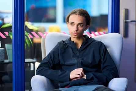






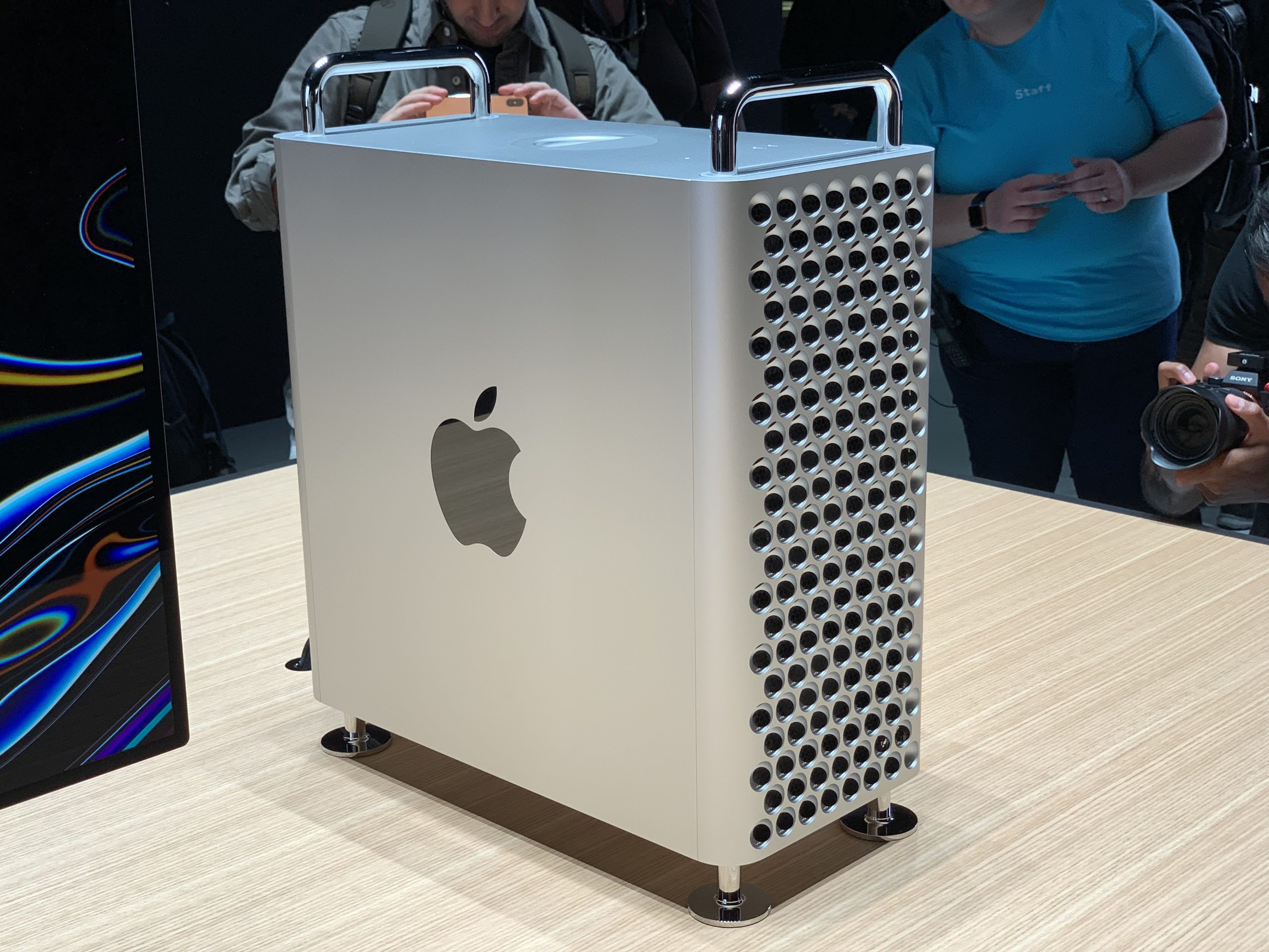
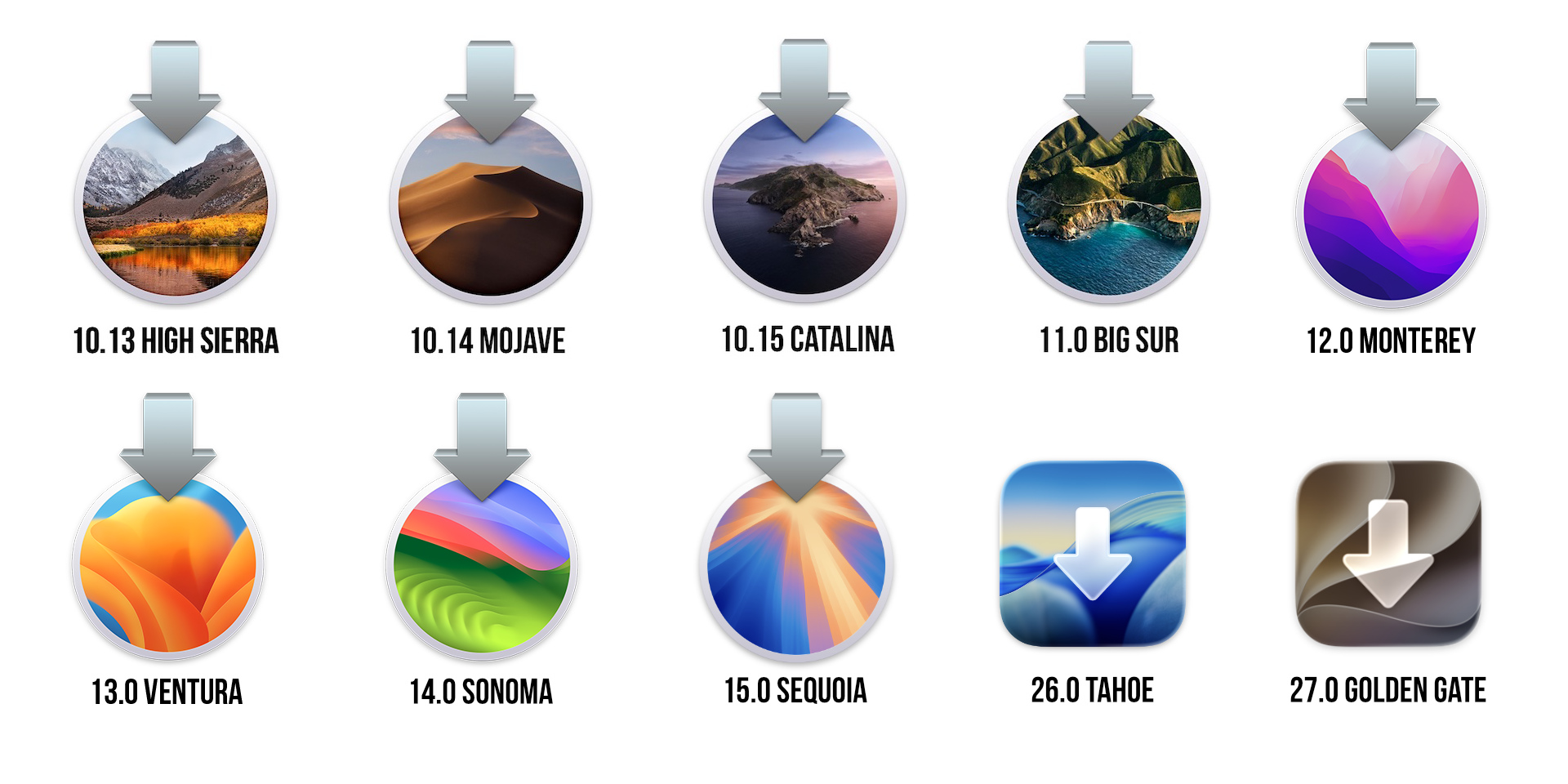

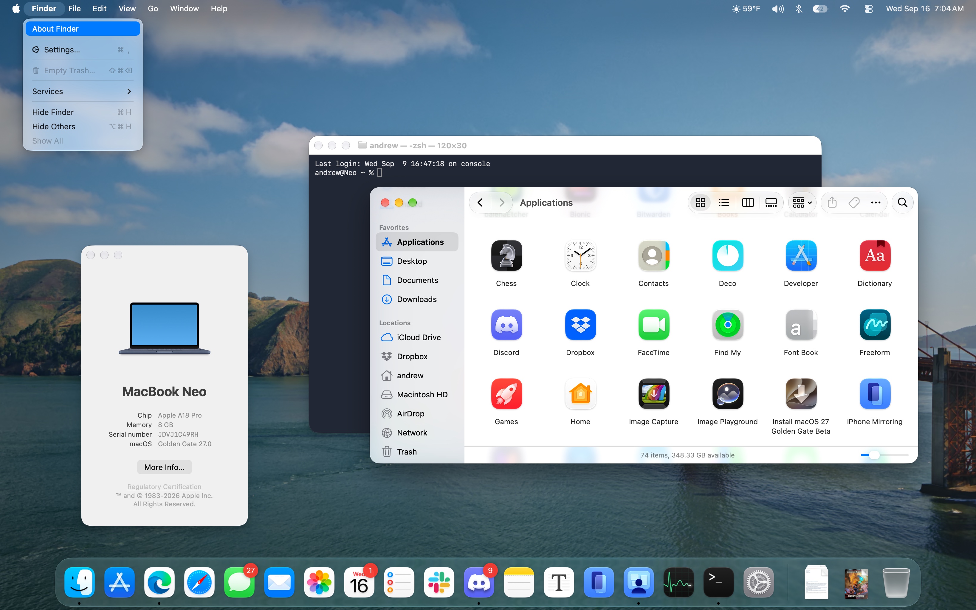
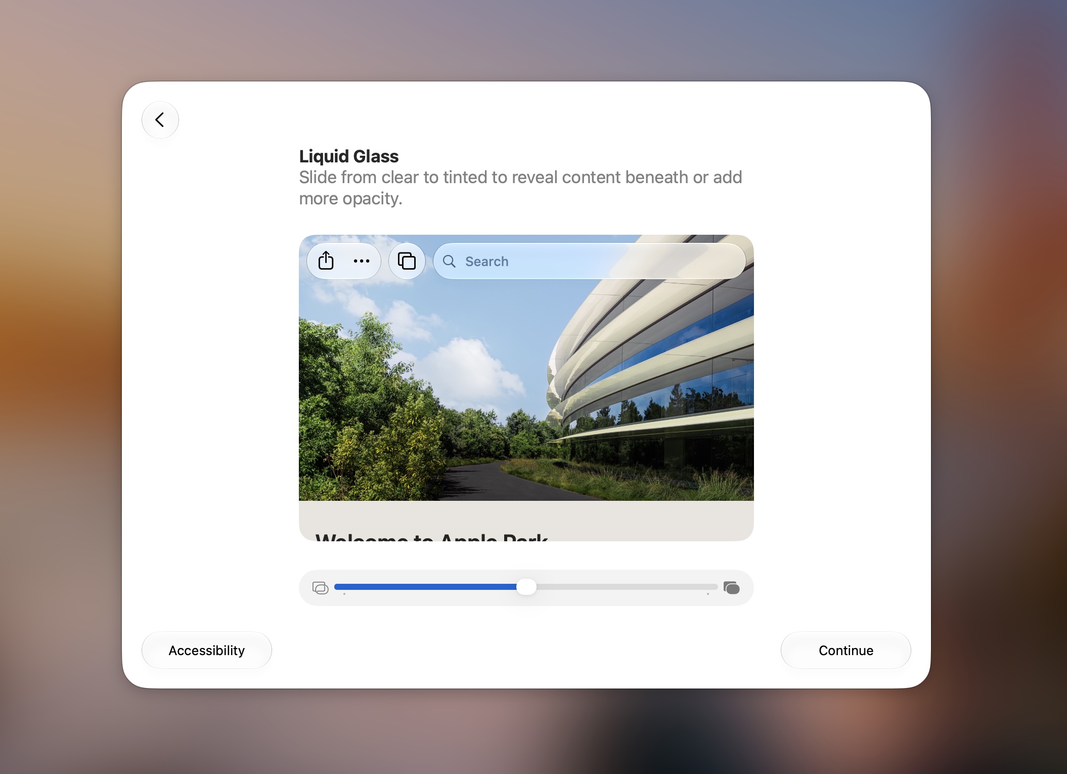
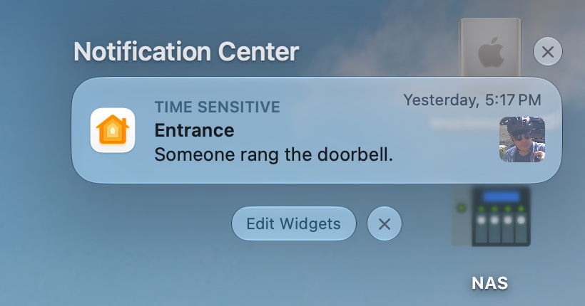
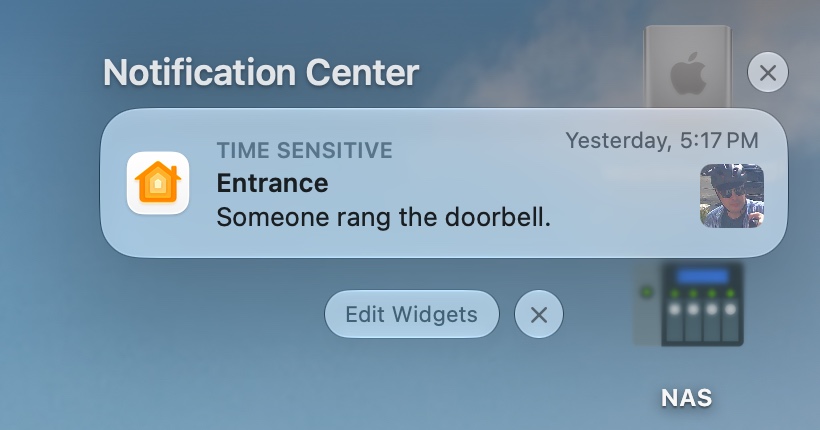
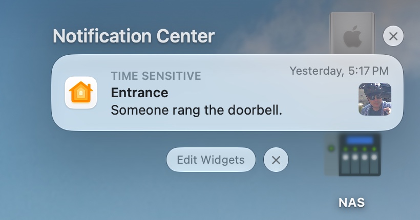
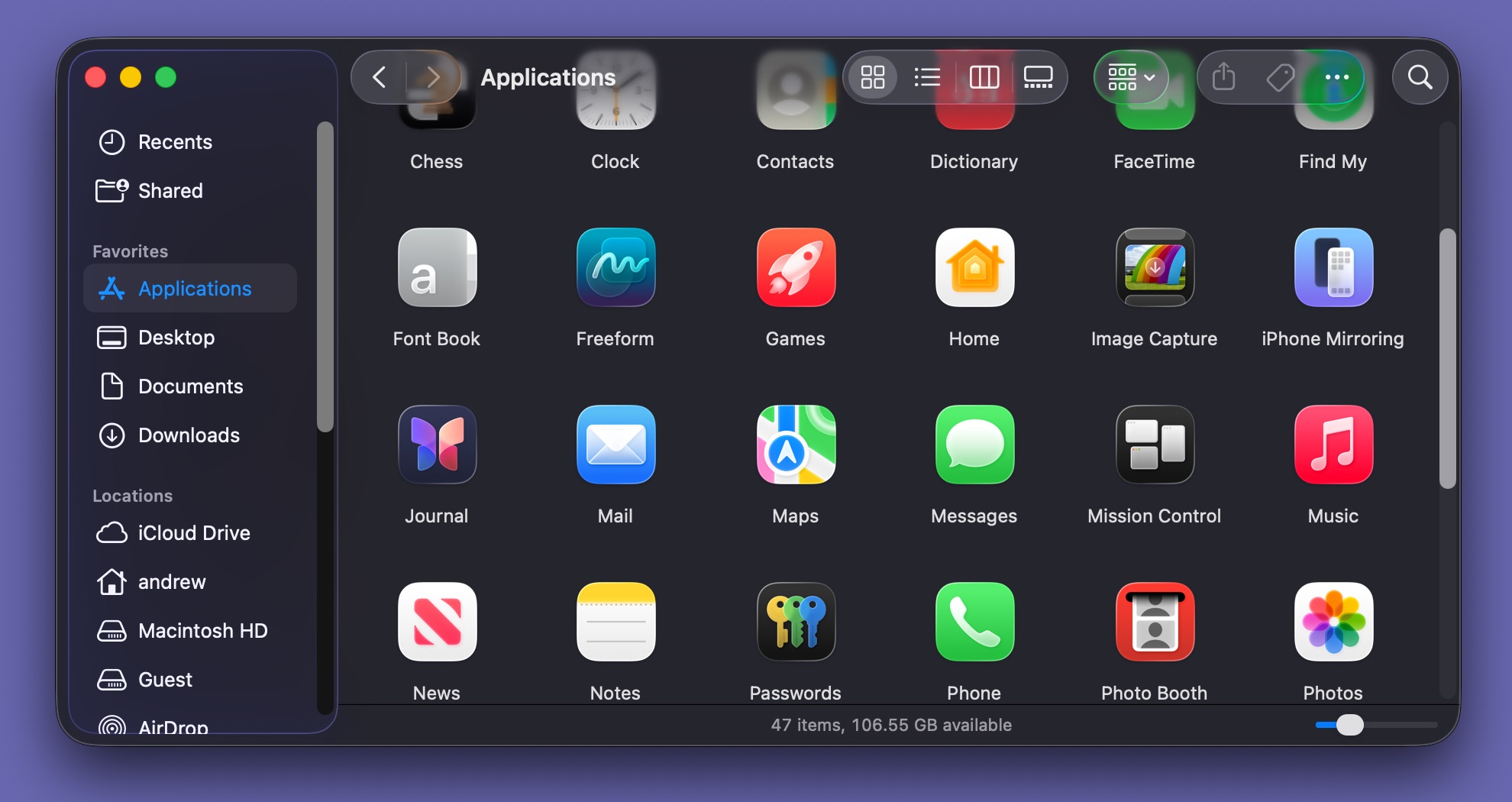
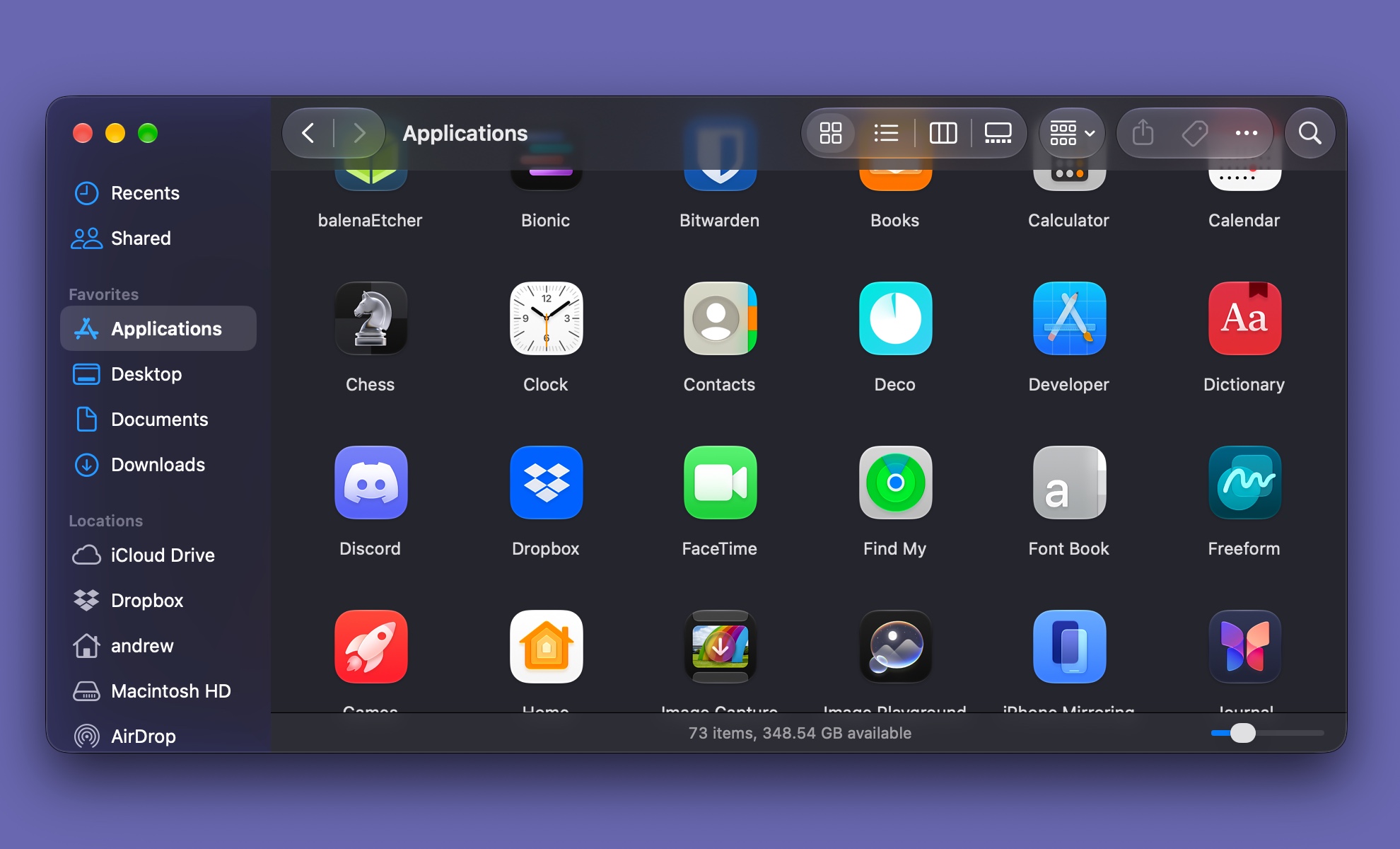
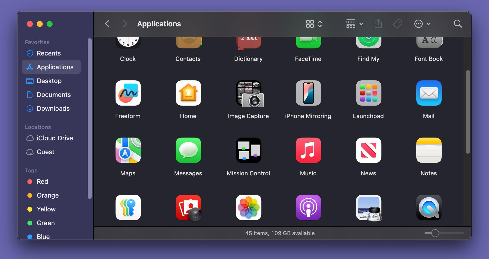
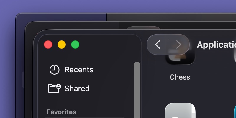
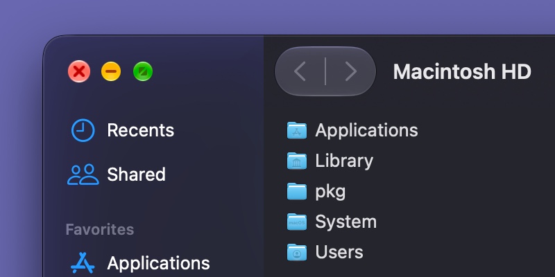
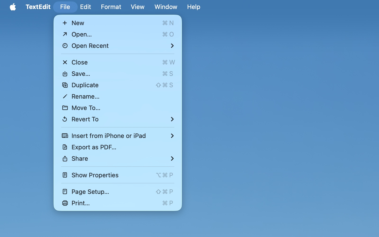
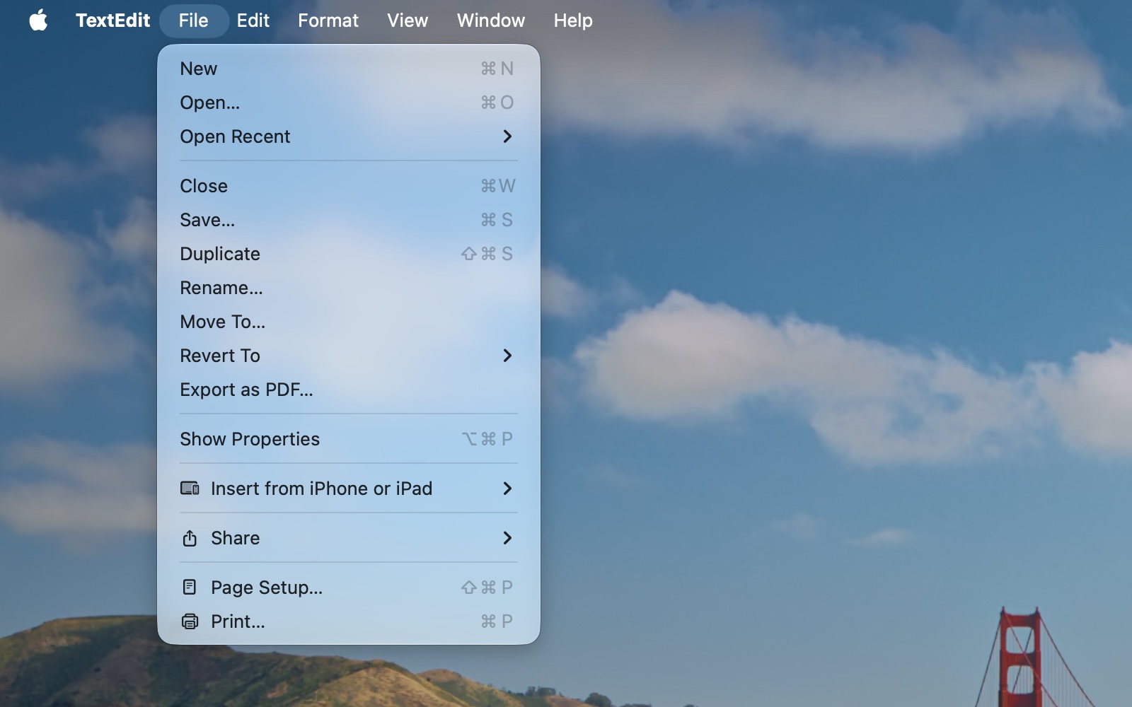
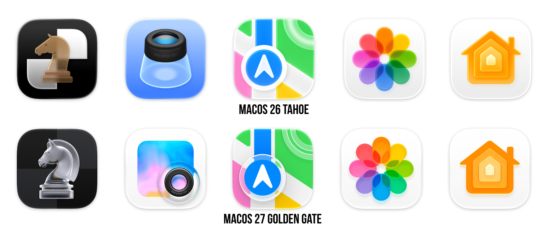

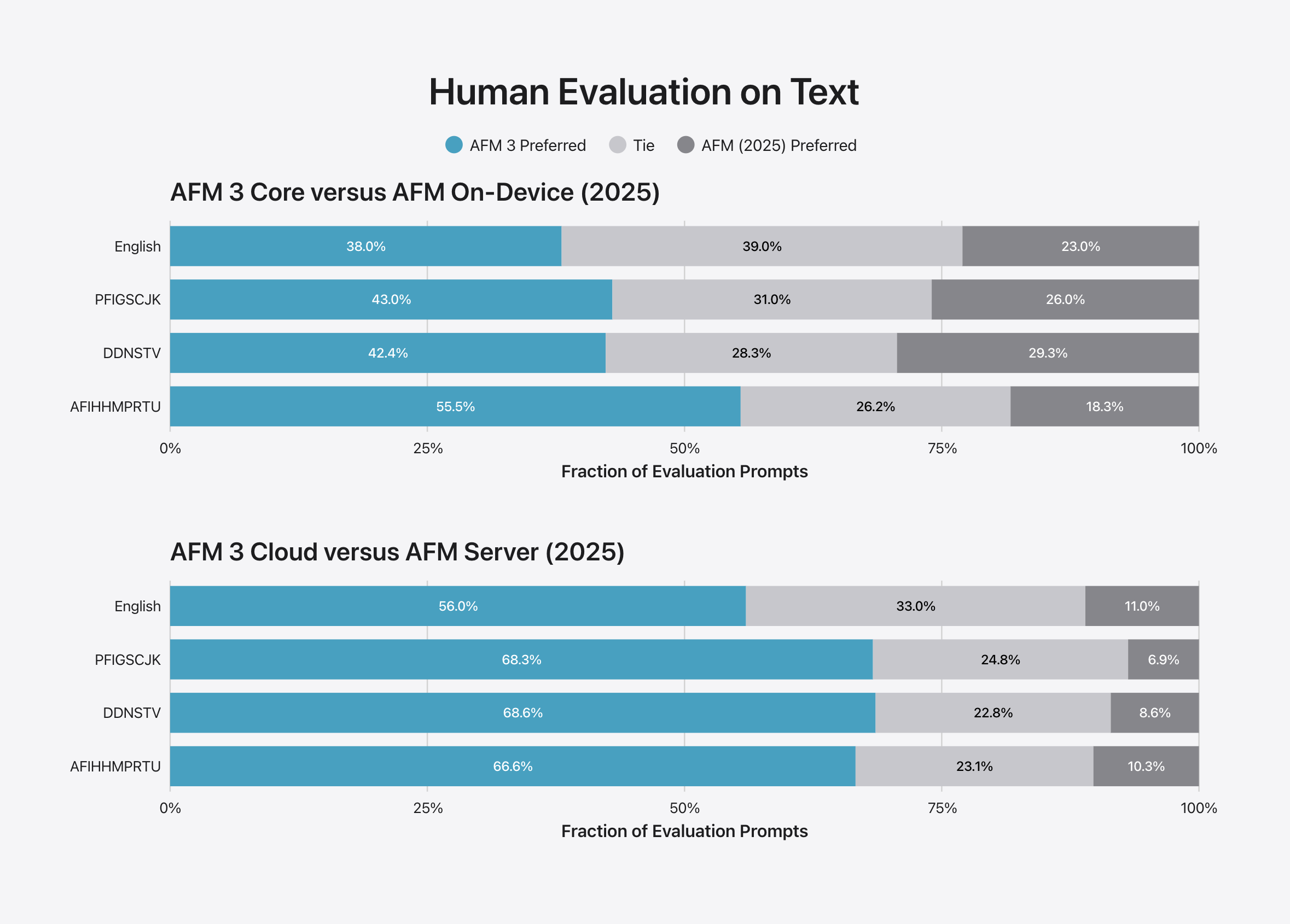
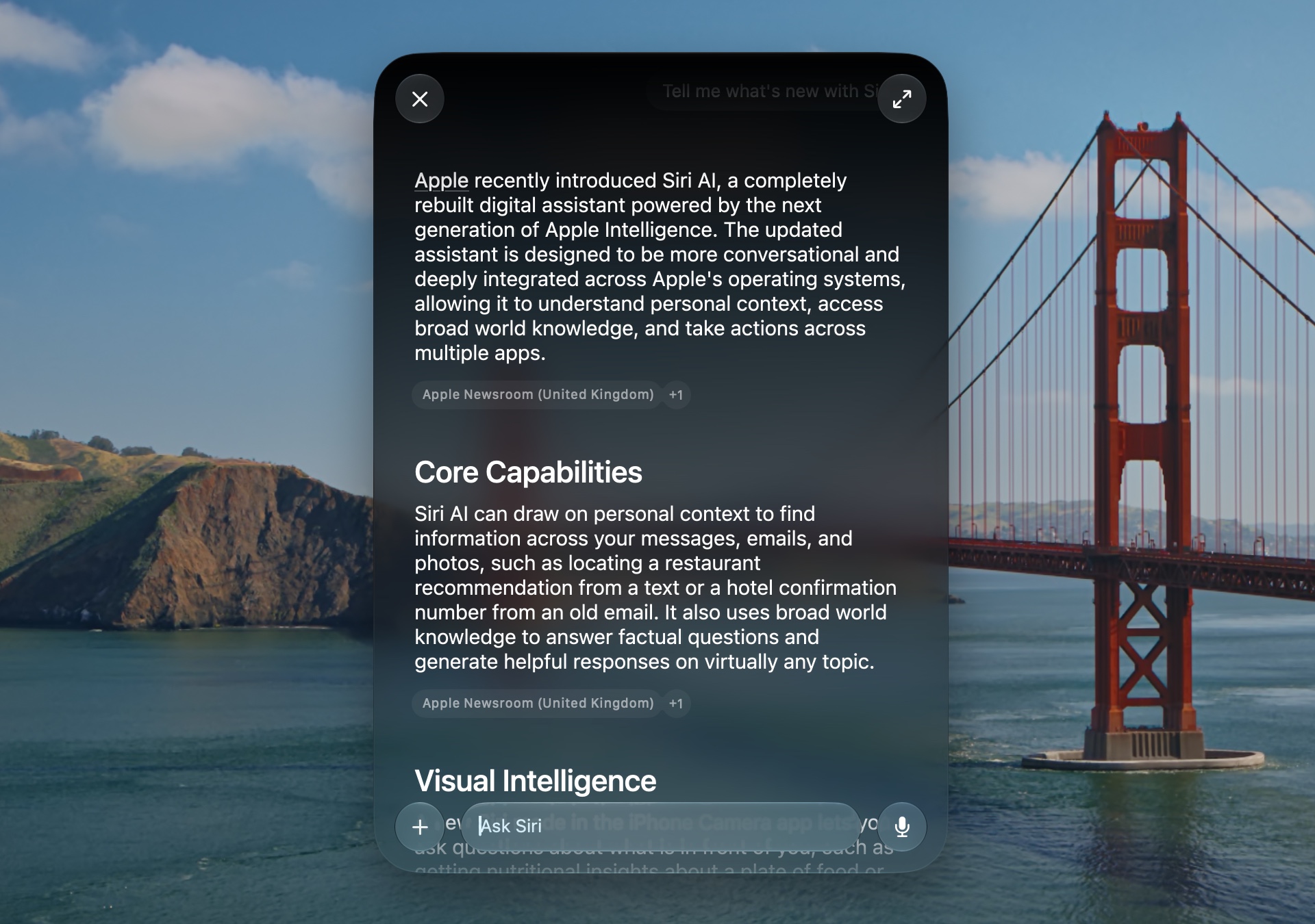
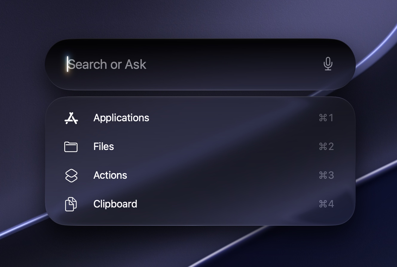
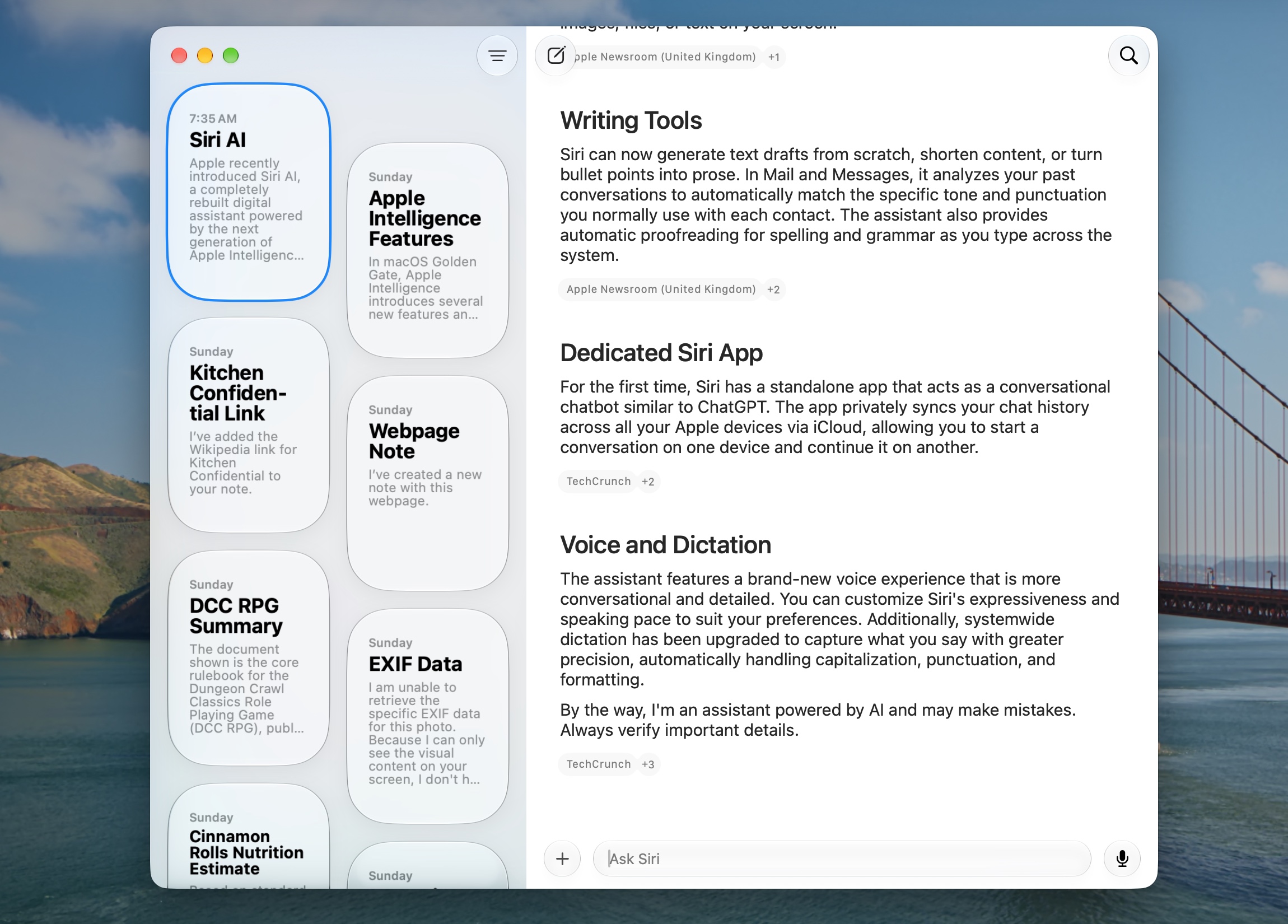
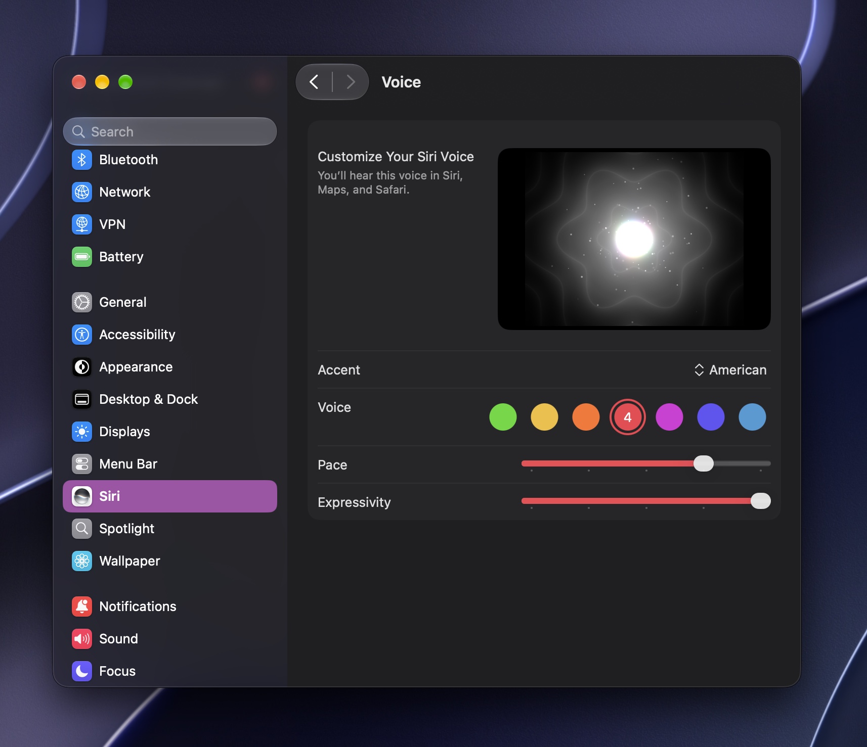
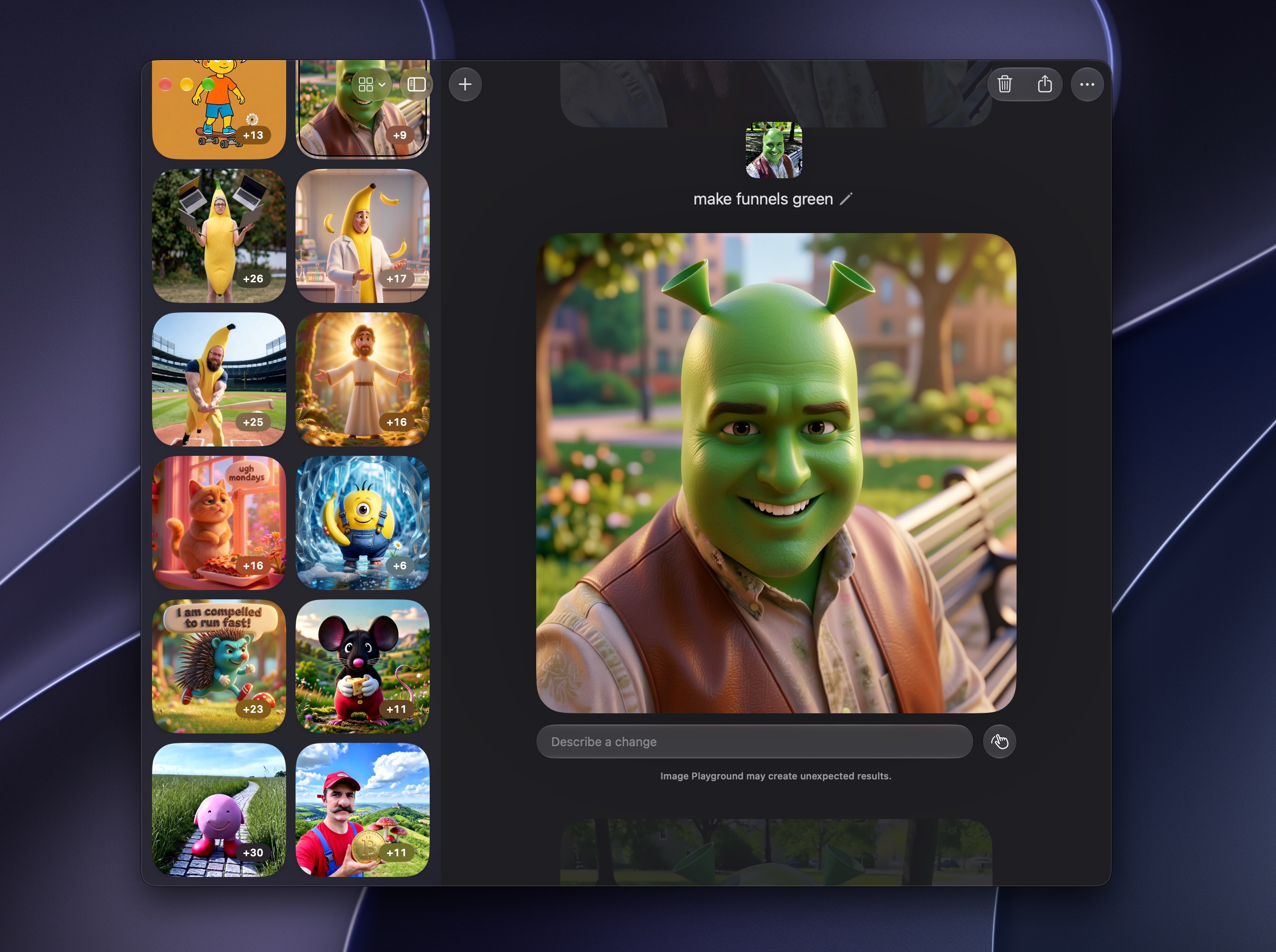
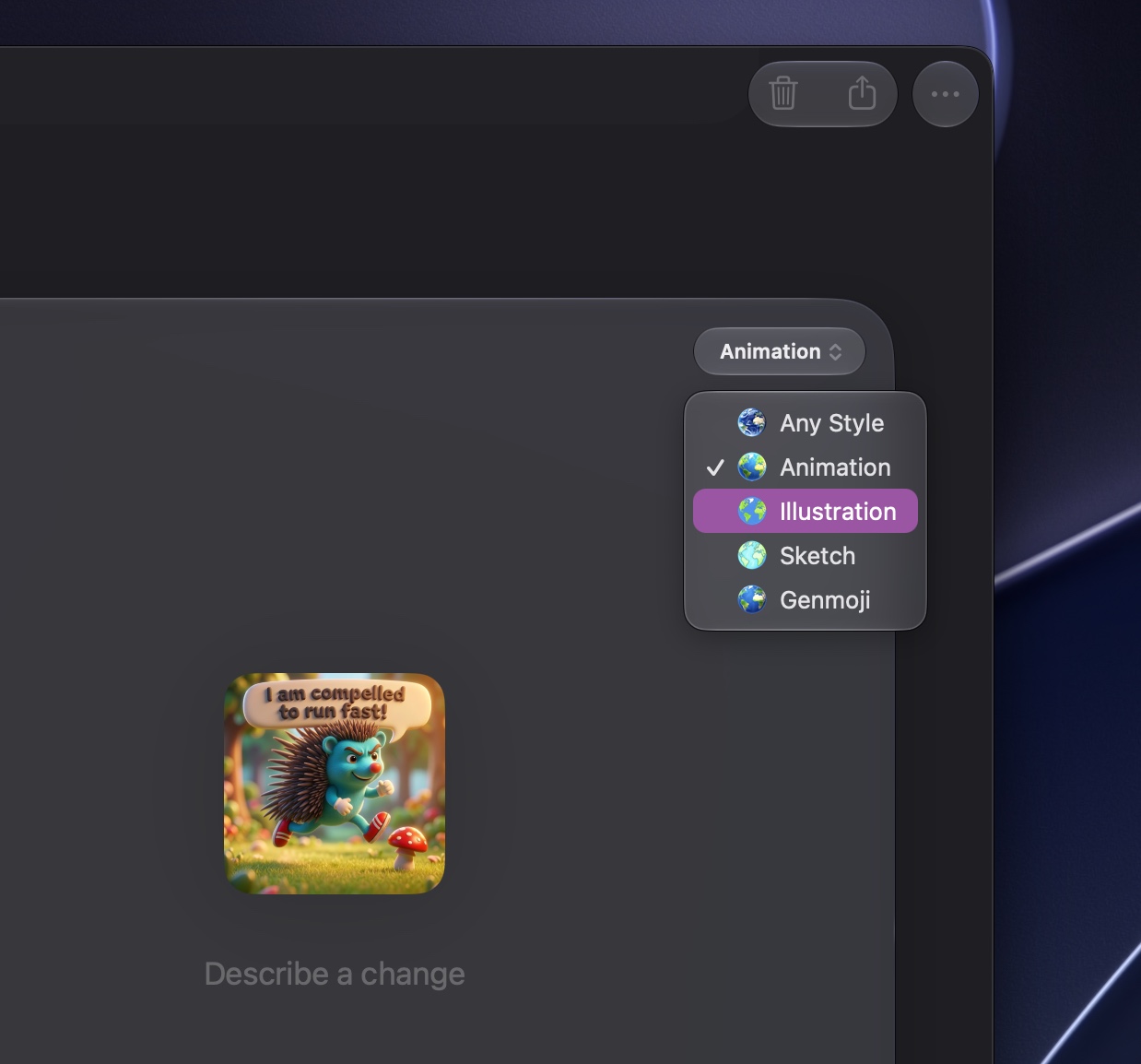


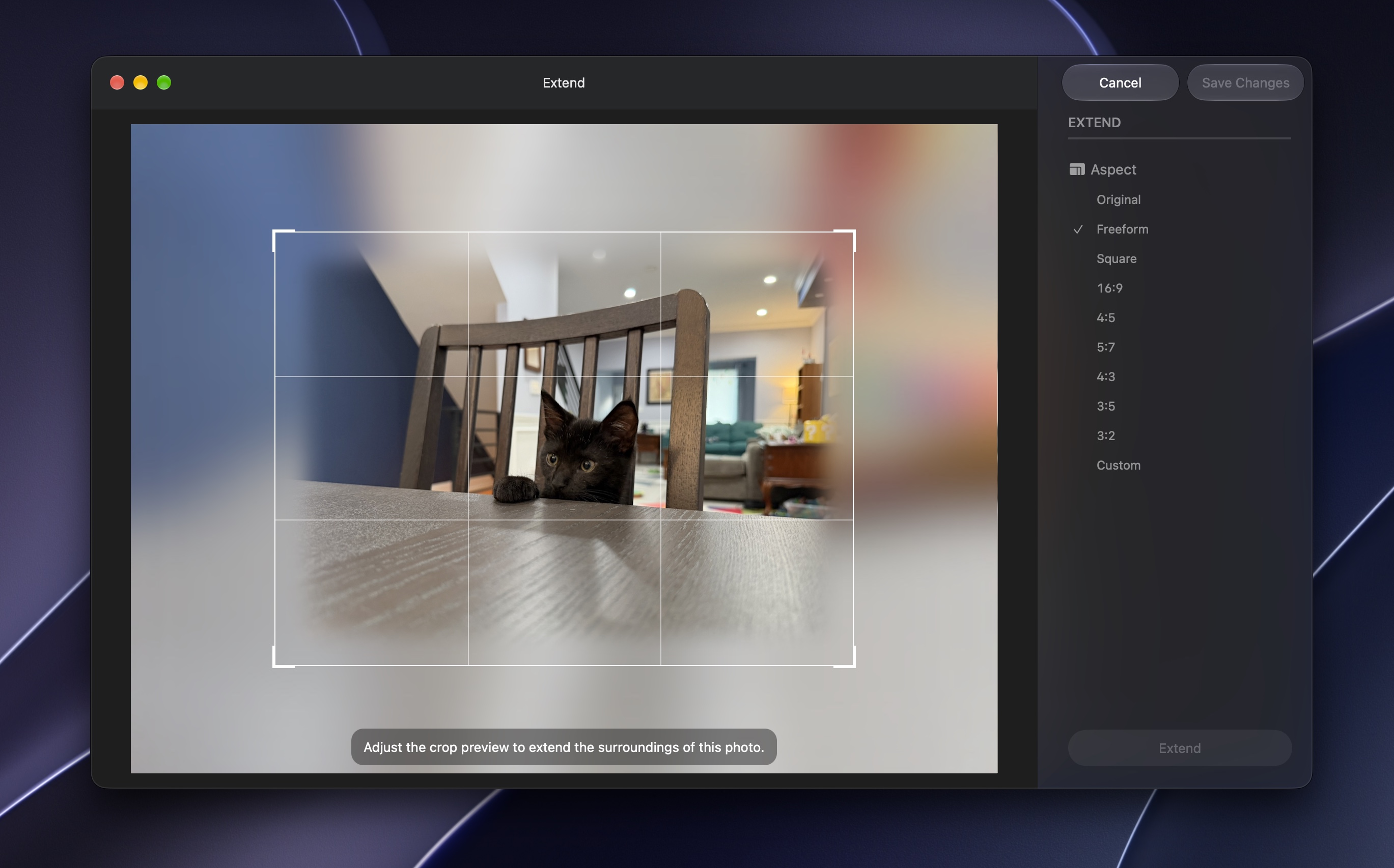
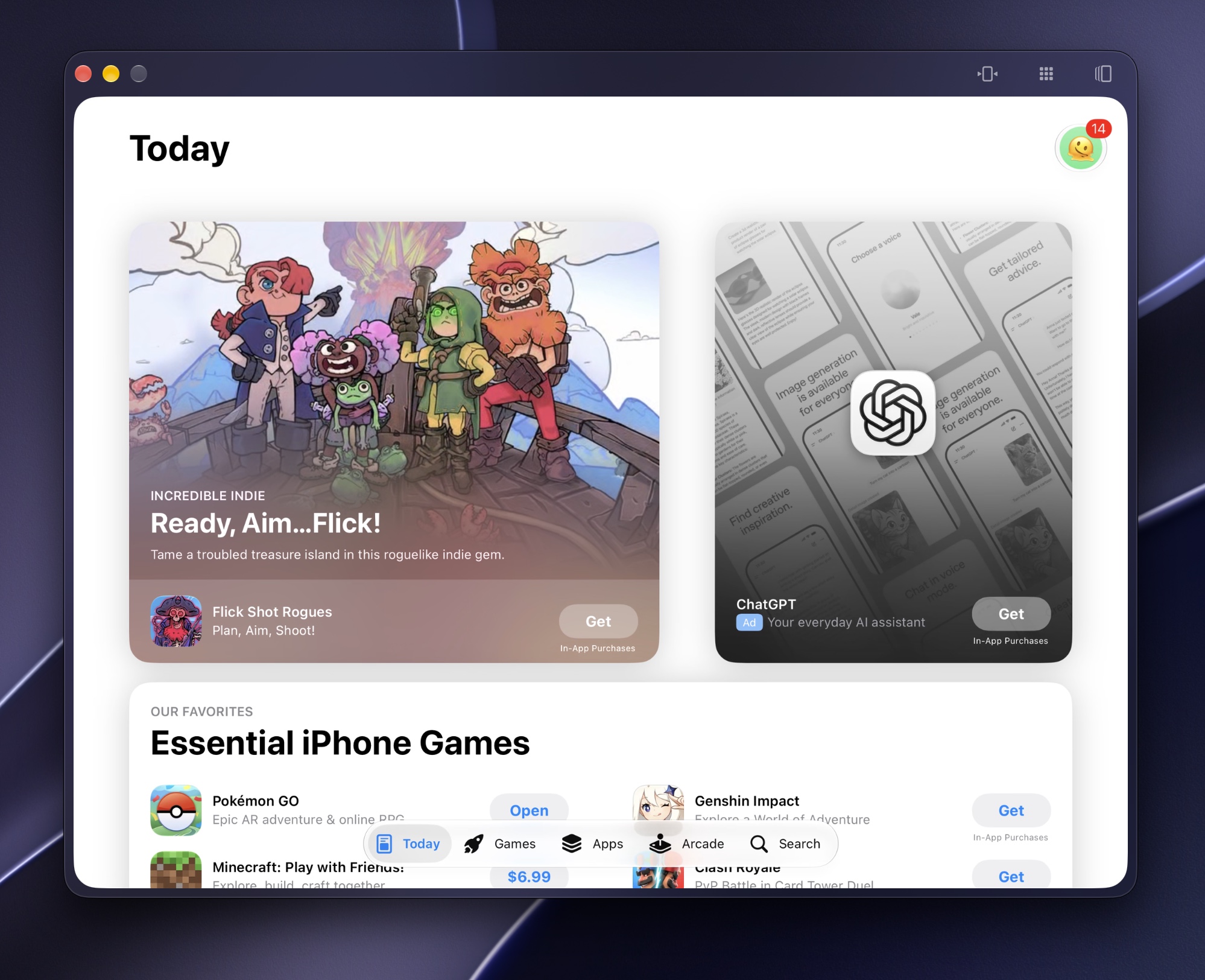
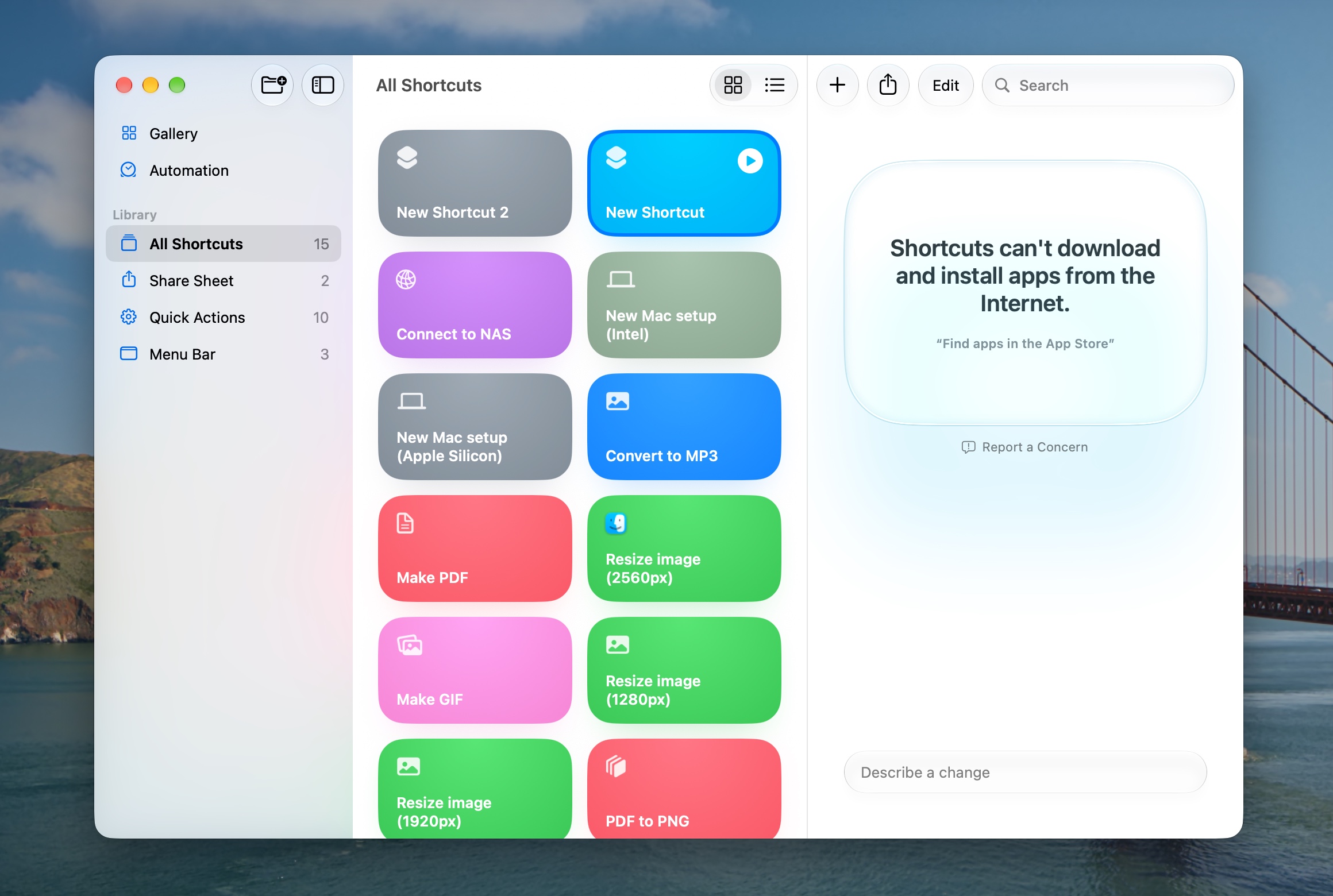
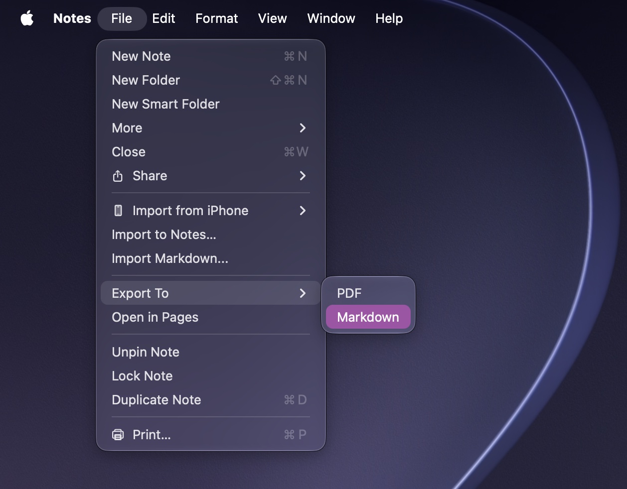
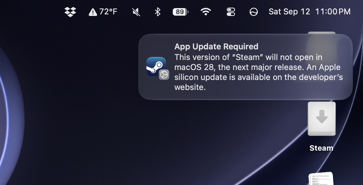
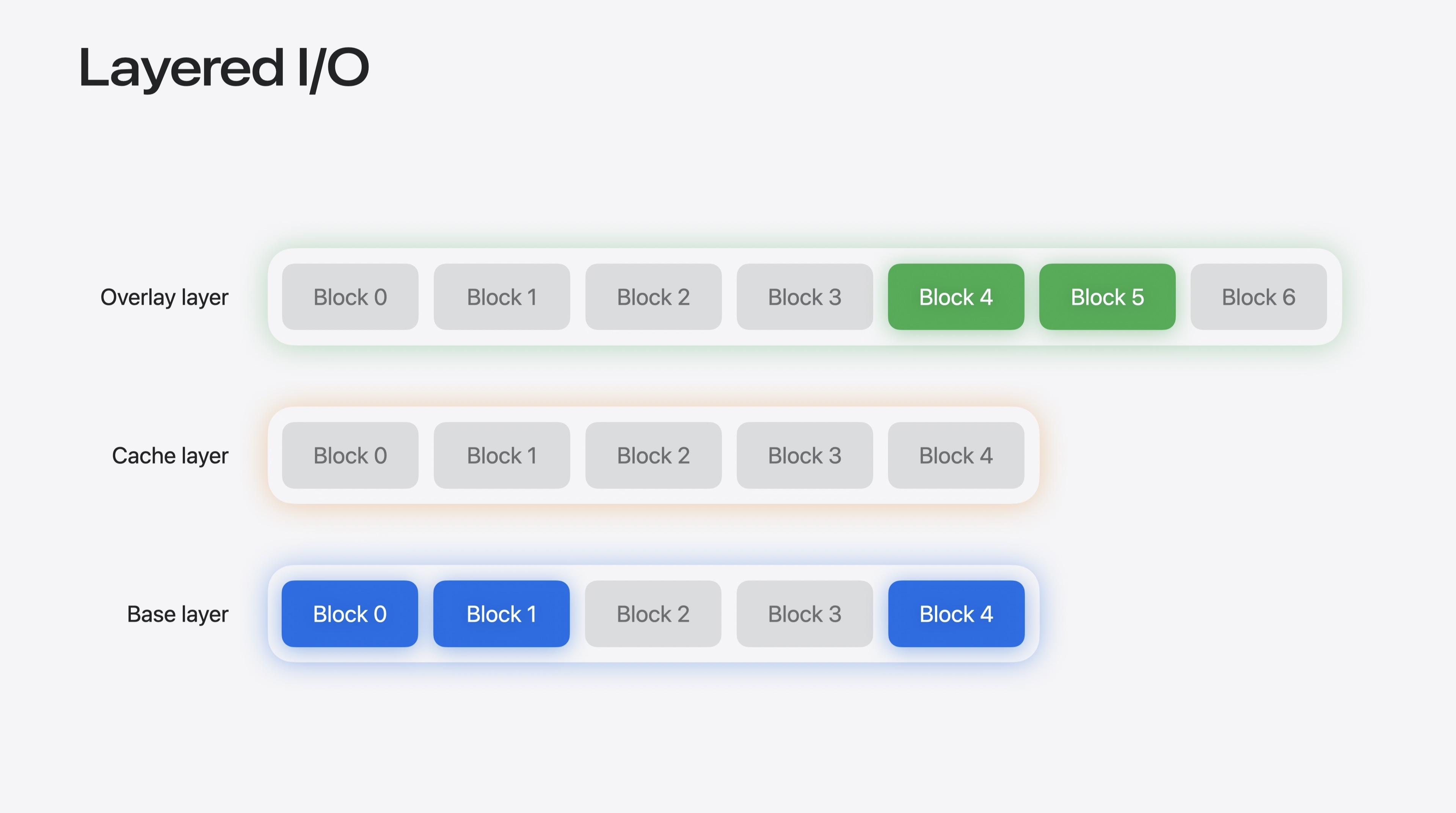
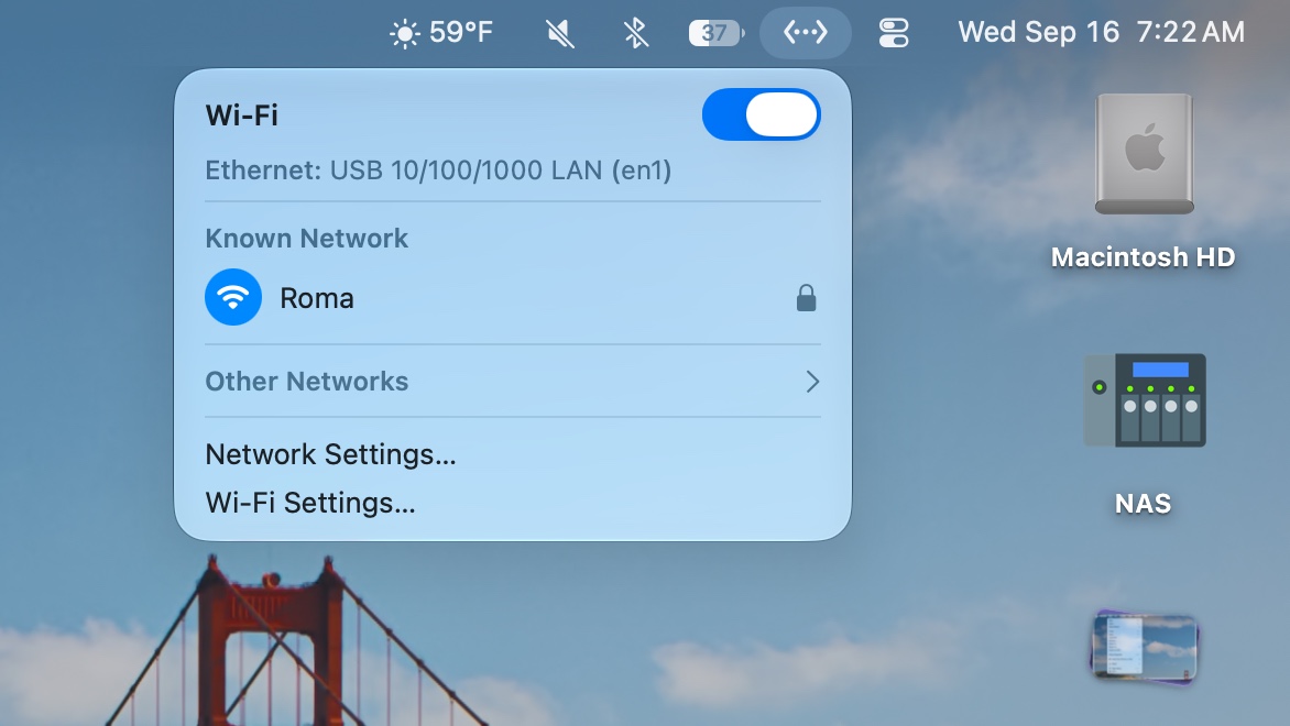
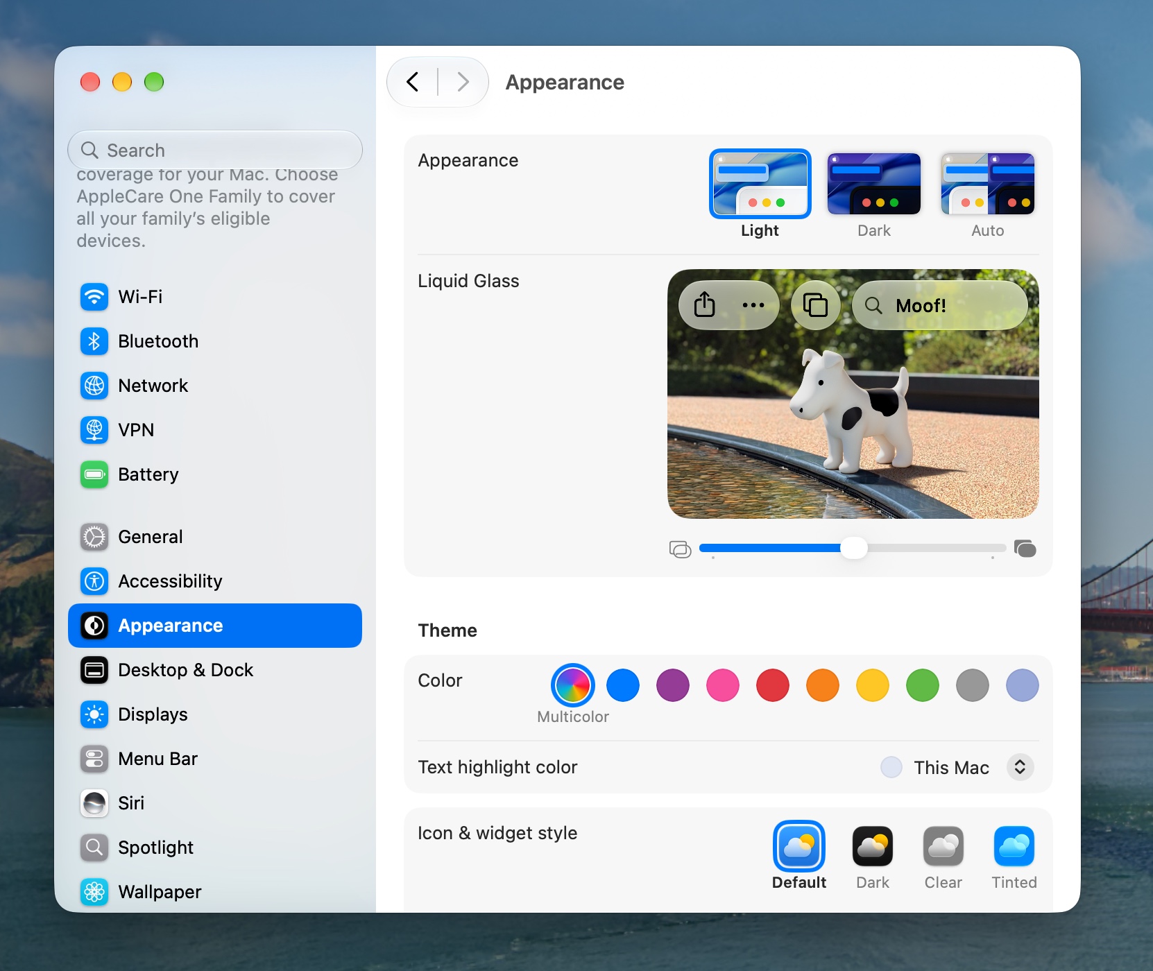

 . This section is a brief overview of how Stirling’s formula is
 is a twice-differentiable function and
  is the global maximum of
  . Moreover:


