Comments

Source: Hacker News

Source: Hacker News

Source: Hacker News

SpaceXAI's most powerful model for coding and knowledge work. Twice as fast, at half the price of comparable models.

Grok 4.7 is our most capable model for coding and knowledge work. It works longer on difficult tasks, checks its own work more carefully, and comes with our best-calibrated safeguards to date. Served at the same price and speed as Grok 4.6, it is highly competitive in its class.

On CursorBench 4.0, which stresses longer-running coding tasks, Grok 4.7 is at the frontier in price-performance.

Grok 4.7 uses a new, larger base model compared to Grok 4.6. It was trained with a longer reinforcement learning run on a harder mix of tasks, weighted toward problems that take many hours to complete. The model is better at verifying its own work and managing longer context. We also trained Grok 4.7 to natively understand the Grok Bot harness, making it better at conversational tasks and general knowledge work.

Grok 4.7 is better at creating documents and presentations. In GDPval and AA Briefcase, AI is asked to work on tasks done by professionals such as lawyers, nurses, and financial analysts. Grok 4.7 improves upon Grok 4.6 on both benchmarks and performs comparably to other frontier models.

Grok 4.7 was built with an entirely new safeguard stack. It is the strongest model we’ve tested on refusals and jailbreak resistance. In dual-use domains like cybersecurity and biological work, it leads on both utility for benign tasks and safe refusal on dangerous ones, topping LatchBio’s biosafety benchmark at 62.4%.

Grok 4.7 balances strong cyber defense capabilities with low refusal rates for legitimate use. It shows the highest safety on HackerBench v0.3, our benchmark for risky and malicious cyber tasks, allowing only 3.3% of risky dual-use prompts through while rarely blocking legitimate security work. We’ve also started giving select cybersecurity partners invite-only access to Grok 4.7’s red-team capabilities for defense research.

Grok 4.7 is available today in Cursor and Grok Build. It is also available through the Grok API, third-party coding harnesses, and model routers and cloud platforms.

The model is priced starting at $2 per million input tokens and $6 per million output tokens. We also serve a fast variant with twice the output speed at twice the price.

Get started today at x.ai/build.

Source: Hacker News

Transformer is a neural network architecture that has fundamentally changed the approach to
Artificial Intelligence. Transformer was first introduced in the seminal paper
"Attention is All You Need"
in 2017 and has since become the go-to architecture for deep learning models, powering text-generative
models like OpenAI's GPT, Meta's Llama, and Google's
Gemini. Beyond text, Transformer is also applied in
audio generation,
image recognition,
protein structure prediction, and even
game playing, demonstrating its versatility across numerous domains.

Fundamentally, text-generative Transformer models operate on the principle of next-token prediction: given a text prompt from the user, what is the
most probable next token (a word or part of a word) that will follow this input? The core
innovation and power of Transformers lie in their use of self-attention mechanism, which allows
them to process entire sequences and capture long-range dependencies more effectively than previous
architectures.

GPT-2 family of models are prominent examples of text-generative Transformers. Transformer
Explainer is powered by the
GPT-2
(small) model which has 124 million parameters. While it is not the latest or most powerful Transformer
model, it shares many of the same architectural components and principles found in the current
state-of-the-art models making it an ideal starting point for understanding the basics.

Every text-generative Transformer consists of these three key components:

Let's say you want to generate text using a Transformer model. You add the prompt like this
one: “Data visualization empowers users to”. This input needs to be converted
into a format that the model can understand and process. That is where embedding comes in: it
transforms the text into a numerical representation that the model can work with. To convert a
prompt into embedding, we need to 1) tokenize the input, 2) obtain token embeddings, 3) add
positional information, and finally 4) add up token and position encodings to get the final
embedding. Let’s see how each of these steps is done.

Tokenization is the process of breaking down the input text into smaller, more manageable
pieces called tokens. These tokens can be a word or a subword. The words "Data"
and "visualization" correspond to unique tokens, while the word
"empowers"
is split into two tokens. The full vocabulary of tokens is decided before training the model:
GPT-2's vocabulary has 50,257 unique tokens. Now that we split our input text into
tokens with distinct IDs, we can obtain their vector representation from embeddings.

GPT-2 (small) represents each token in the vocabulary as a 768-dimensional vector; the
dimension of the vector depends on the model. These embedding vectors are stored in a matrix
of shape (50,257, 768), containing approximately 39 million parameters! This
extensive matrix allows the model to assign semantic meaning to each token, in the sense
that tokens with similar usage or meaning in language are placed close together in this
high-dimensional space, while dissimilar tokens are farther apart.

The Embedding layer also encodes information about each token's position in the input
prompt. Different models use various methods for positional encoding. GPT-2 trains its own
positional encoding matrix from scratch, integrating it directly into the training process.

Finally, we sum the token and positional encodings to get the final embedding
representation. This combined representation captures both the semantic meaning of the
tokens and their position in the input sequence.

The core of the Transformer's processing lies in the Transformer block, which comprises
multi-head self-attention and a Multi-Layer Perceptron layer. Most models consist of multiple
such blocks that are stacked sequentially one after the other. The token representations
evolve through layers, from the first block to the last one, allowing the model to build up an
intricate understanding of each token. This layered approach leads to higher-order
representations of the input. The GPT-2 (small) model we are examining consists of 12 such blocks.

The self-attention mechanism enables the model to capture relationships among tokens in a
sequence, so that each token’s representation is influenced by the others. Multiple attention
heads allow the model to consider these relationships from different perspectives; for
example, one head may capture short-range syntactic links while another tracks broader
semantic context. In the following section, we will walk through how multi-head self-attention
is computed step by step.

Each token's embedding vector is transformed into three vectors:
Query (Q),
Key (K), and
Value (V). These vectors are derived by multiplying the input
embedding matrix with learned weight matrices for
Q,
K, and
V. Here's a web search analogy to help us build some intuition
behind these matrices:

By using these QKV values, the model can calculate attention scores, which determine how
much focus each token should receive when generating predictions.

Query, key, and
Value
vectors are split into multiple heads—in GPT-2 (small)'s case, into
12 heads. Each head processes a segment of the embeddings independently, capturing
different syntactic and semantic relationships. This design facilitates parallel learning of
diverse linguistic features, enhancing the model's representational power.

In each head, we perform masked self-attention calculations. This mechanism allows the model
to generate sequences by focusing on relevant parts of the input while preventing access to
future tokens.

The model uses the masked self-attention scores and multiplies them with the
Value matrix to get the
final output
of the self-attention mechanism. GPT-2 has 12 self-attention heads, each capturing
different relationships between tokens. The outputs of these heads are concatenated and passed
through a linear projection.

After the multiple heads of self-attention capture the diverse relationships between the input
tokens, the concatenated outputs are passed through the Multilayer Perceptron (MLP) layer to
enhance the model's representational capacity. The MLP block consists of two linear
transformations with a GELU activation function in between.

The first linear transformation expands the dimensionality of the input four-fold from 768
to
3072. This expansion step allows the model to project the token representations
into a higher-dimensional space, where it can capture richer and more complex patterns that
may not be visible in the original dimension.

The second linear transformation then reduces the dimensionality back to the original size of 768.This compression step brings the representations back to a manageable size while retaining
the useful nonlinear transformations introduced in the expansion step.

Unlike the self-attention mechanism, which integrates information across tokens, the MLP
processes tokens independently and simply maps each token representation from one space to
another, enriching the overall model capacity.

After the input has been processed through all Transformer blocks, the output is passed
through the final linear layer to prepare it for token prediction. This layer projects the
final representations into a 50,257
dimensional space, where every token in the vocabulary has a corresponding value called
logit. Any token can be the next word, so this process allows us to simply rank
these tokens by their likelihood of being that next word. We then apply the softmax function
to convert the logits into a probability distribution that sums to one. This will allow us to
sample the next token based on its likelihood.

The final step is to generate the next token by sampling from this distribution The temperature
hyperparameter plays a critical role in this process. Mathematically speaking, it is a very simple
operation: model output logits are simply divided by the
temperature:

In addition, the sampling process can be further refined using top-k
and
top-p parameters:

By tuning temperature, top-k, and top-p, you can
balance between deterministic and diverse outputs, tailoring the model's behavior to your
specific needs.

There are several auxiliary architectural features that enhance the performance of Transformer
models. While important for the model's overall performance, they are not as important for
understanding the core concepts of the architecture. Layer Normalization, Dropout, and
Residual Connections are crucial components in Transformer models, particularly during the
training phase. Layer Normalization stabilizes training and helps the model converge faster.
Dropout prevents overfitting by randomly deactivating neurons. Residual Connections allows
gradients to flow directly through the network and helps to prevent the vanishing gradient
problem.

Layer Normalization helps to stabilize the training process and improves convergence. It
works by normalizing the inputs across the features, ensuring that the mean and variance of
the activations are consistent. This normalization helps mitigate issues related to internal
covariate shift, allowing the model to learn more effectively and reducing the sensitivity
to the initial weights. Layer Normalization is applied twice in each Transformer block, once
before the self-attention mechanism and once before the MLP layer.

Dropout is a regularization technique used to prevent overfitting in neural networks by
randomly setting a fraction of model weights to zero during training. This encourages the
model to learn more robust features and reduces dependency on specific neurons, helping the
network generalize better to new, unseen data. During model inference, dropout is
deactivated. This essentially means that we are using an ensemble of the trained
subnetworks, which leads to a better model performance.

Residual connections were first introduced in the ResNet model in 2015. This architectural
innovation revolutionized deep learning by enabling the training of very deep neural
networks. Essentially, residual connections are shortcuts that bypass one or more layers,
adding the input of a layer to its output. This helps mitigate the vanishing gradient
problem, making it easier to train deep networks with multiple Transformer blocks stacked on
top of each other. In GPT-2, residual connections are used twice within each Transformer
block: once before the MLP and once after, ensuring that gradients flow more easily, and
earlier layers receive sufficient updates during backpropagation.

Transformer Explainer is built to be interactive and allows you to explore the inner workings
of the Transformer. Here are some of the interactive features you can play with:

Transformer Explainer features a live GPT-2 (small) model running directly in the browser.
This model is derived from the PyTorch implementation of GPT by Andrej Karpathy's
nanoGPT project
and has been converted to
ONNX Runtime
for seamless in-browser execution. The interface is built using JavaScript, with
Svelte
as a front-end framework and
D3.js
for creating dynamic visualizations. Numerical values are updated live following the user input.

Transformer Explainer was created by

Aeree Cho,
Grace C. Kim,
Alexander Karpekov,
Alec Helbling,
Jay Wang,
Seongmin Lee,
Benjamin Hoover, and
Polo Chau

at the Georgia Institute of Technology.

Source: Hacker News

Comments

Source: Hacker News

1. Now
2. From the team

AI coding has made CI a bottleneck, so we reworked ours to keep up

Mufeez Amjad

·September 21, 2026

Earlier this year, I opened Linear to find that Tuomas, our CTO, had assigned an issue to me, titled “CI costs are high.” While I was at it, he also wanted me to make CI faster.

Agents have made it exponentially faster to ship code, but validating those changes hasn’t quite kept up at the same rate. Every PR still has to pass through CI, so as development accelerates, CI becomes a bottleneck, driving up infrastructure costs and leaving developers and agents waiting longer for feedback.

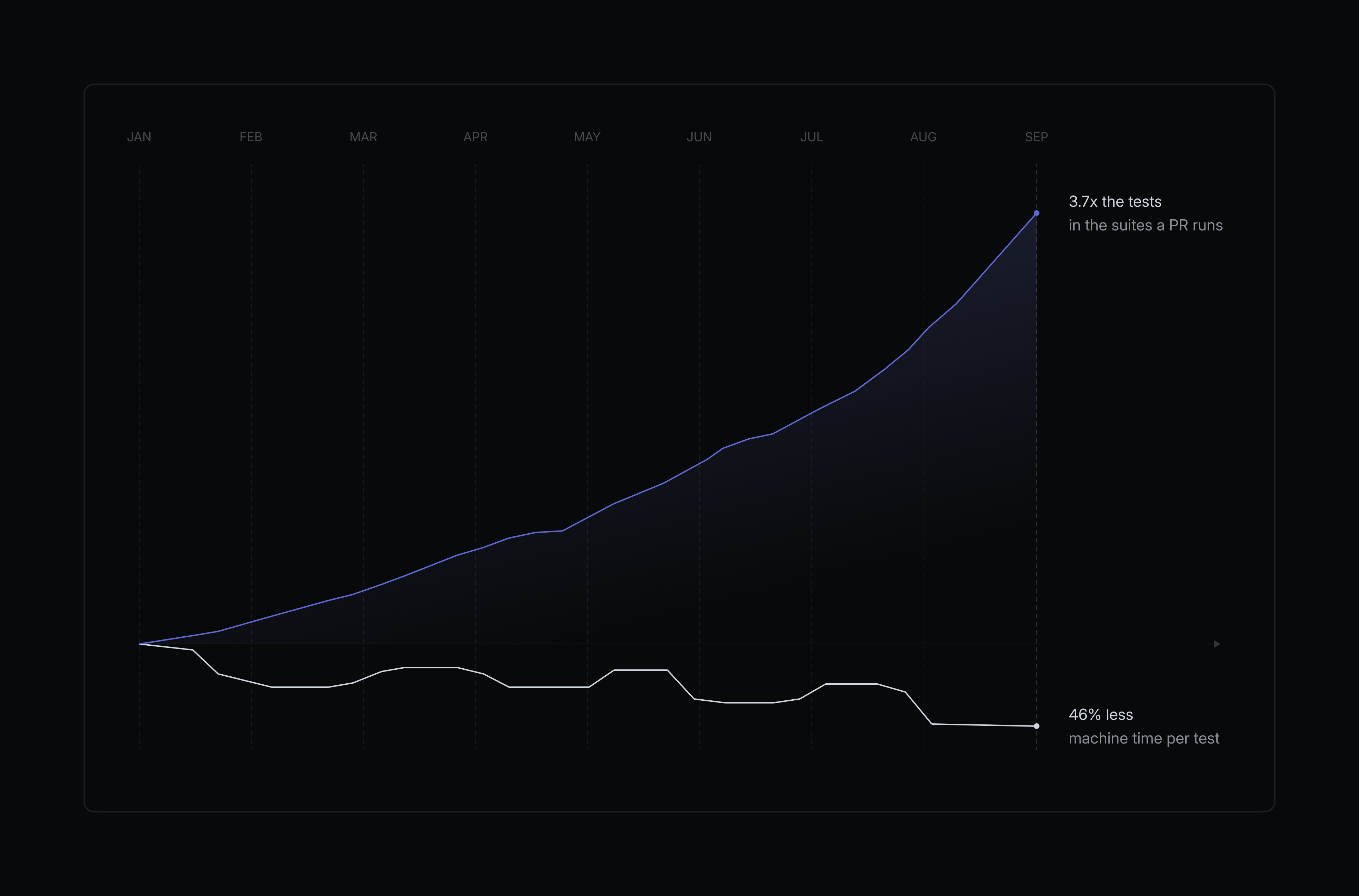
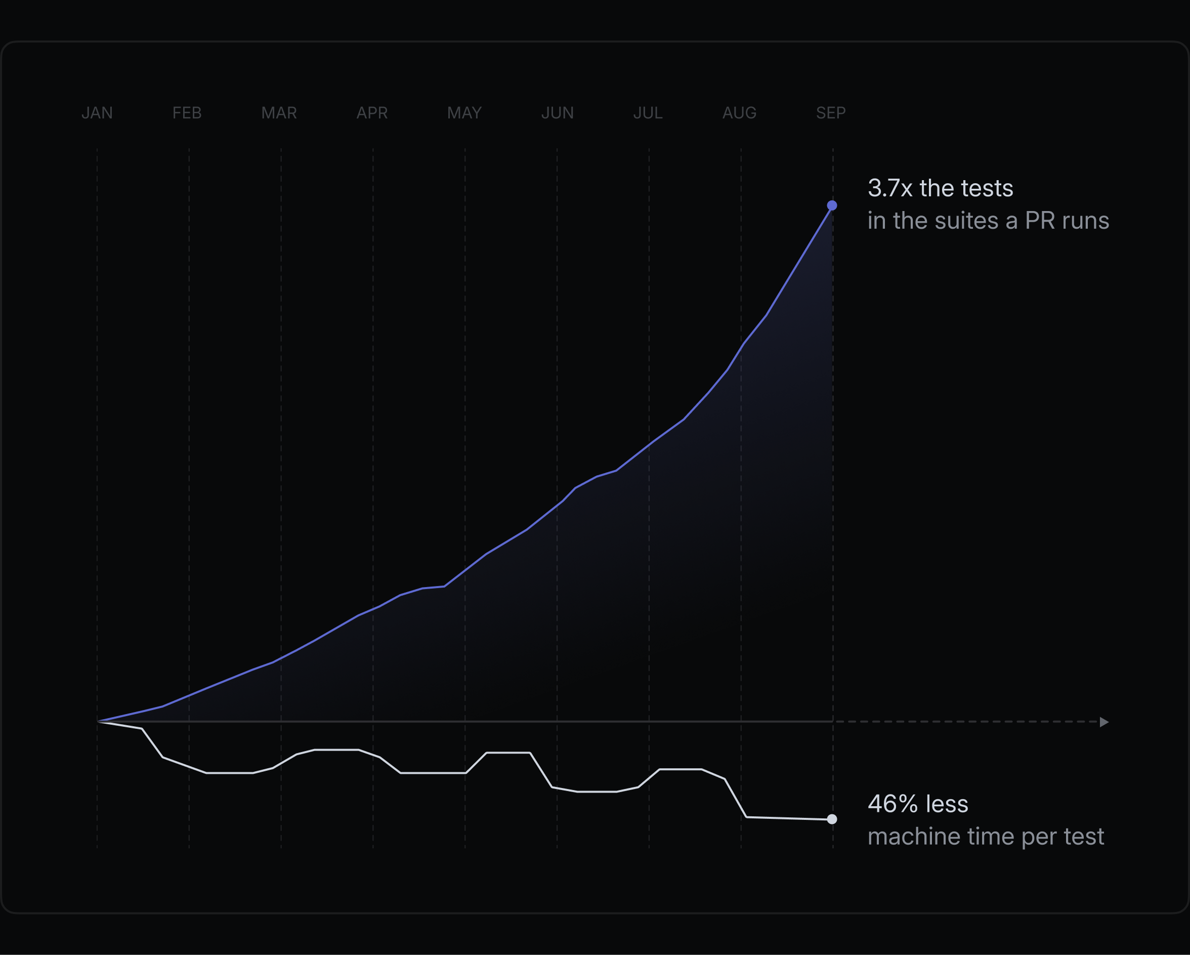
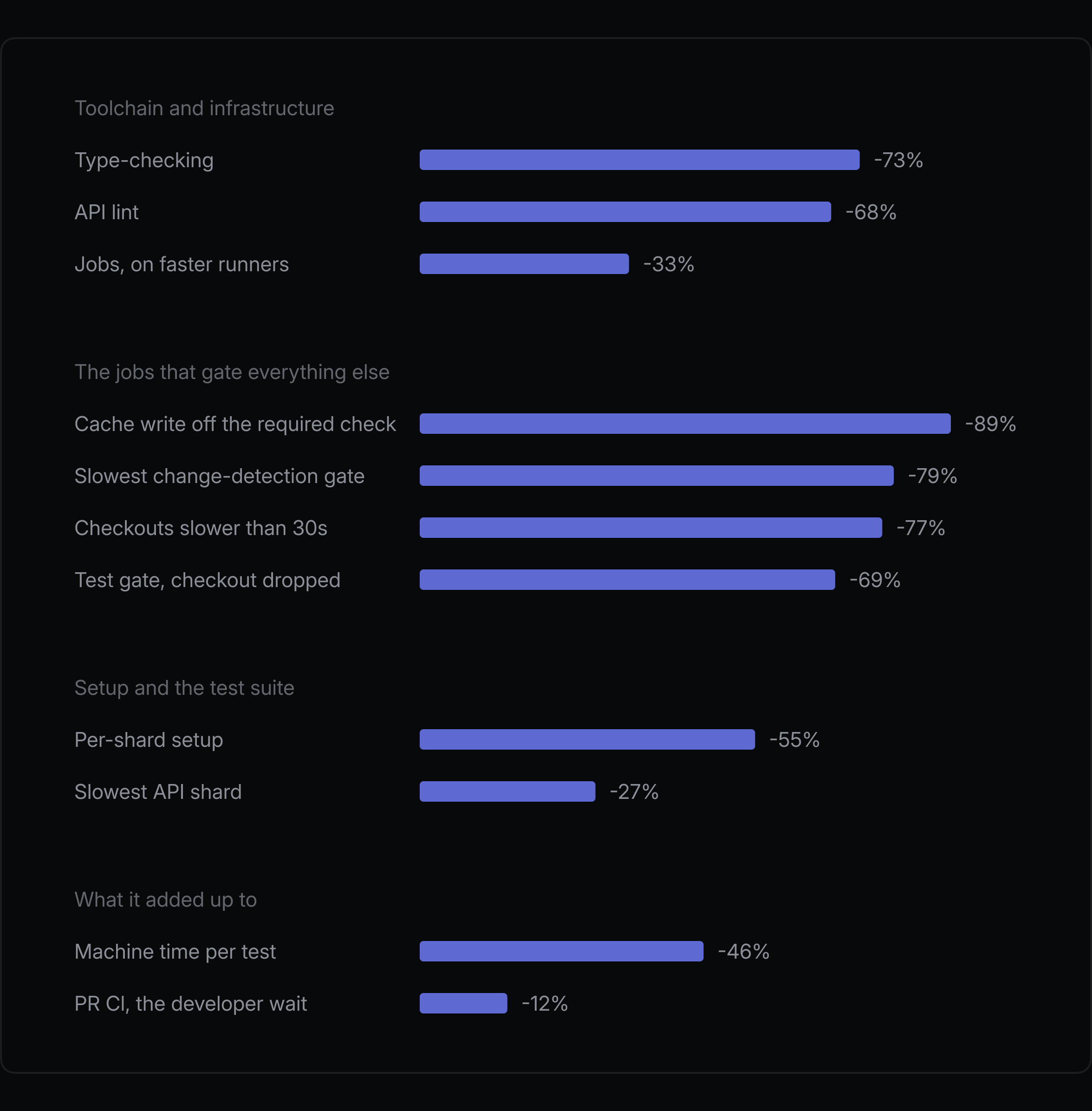
In our pursuit to make CI more performant at Linear, we optimized for how long a PR waits on CI and how much runner time it consumes. Despite our test suites almost quadrupling since the start of the year, we brought pull request wait time down from more than 6 minutes to just over 5, while cutting runner time per test roughly in half.

Broadly, we improved CI in four ways:

• Upgraded infrastructure and tooling
• Optimized the jobs that gate other work
• Reduced repeated setup
• Made test execution more efficient

Linear’s codebase is primarily TypeScript, but many of these optimizations apply across languages and toolchains.

Upgraded infrastructure and tooling⁠

Some of our earliest gains required almost no optimization of CI itself. Moving our workloads off GitHub Actions to third-party runners with faster CPUs, higher-performance storage, and better cache infrastructure gave us faster machines to run the same pipeline on. In a like-for-like comparison of the two days either side of the switch, jobs ran 34% faster on average, with some workloads like tsc dropping 52%.

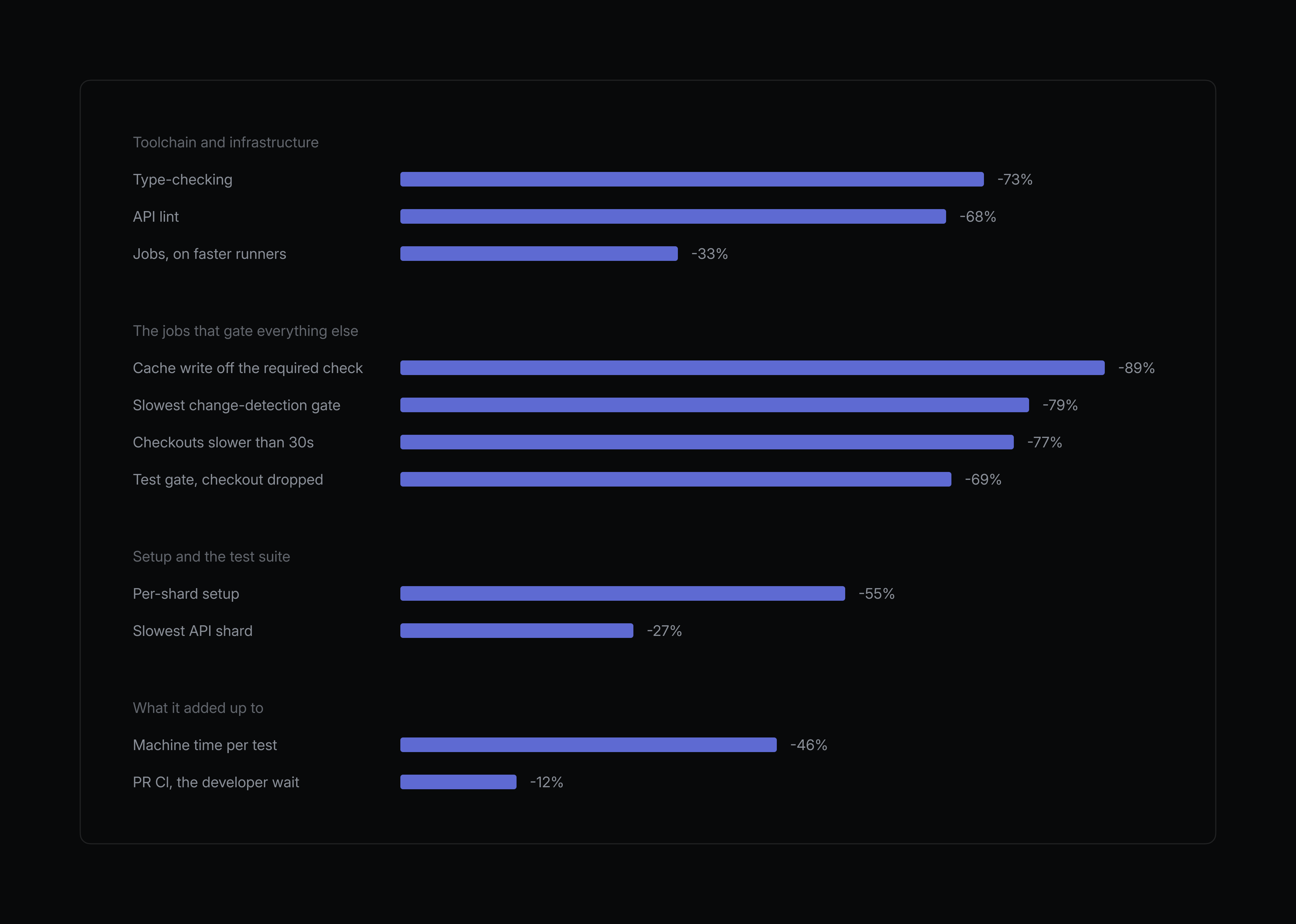
Separately, modernizing our toolchain also paid off. Switching to tsgo, the native TypeScript compiler, cut the weekly median of the tsc check by 73%, large enough to move the bottleneck off of typechecking entirely.

Lint without the type checker⁠

Linting was another early target. A handful of our custom lint rules depended on TypeScript type information, either to enforce a restriction or apply an autofix. That meant every lint run had to build the full type graph before evaluating those rules, making linting one of our most memory-intensive CI jobs.

We rewrote the rules to use static analysis over the abstract syntax tree, identifying function-like constructs and guard patterns without type information. That let ESLint drop TypeScript entirely, reducing API lint time by 68%, and full-repository lint time by 55%. Memory usage dropped substantially as well.

Removing the dependency on type information also made our later move to Oxlint much easier because rules that operate purely on syntax are straightforward to port. Oxlint itself reduced the CI runner-minutes spent on linting.

Optimize the jobs that gate other work⁠

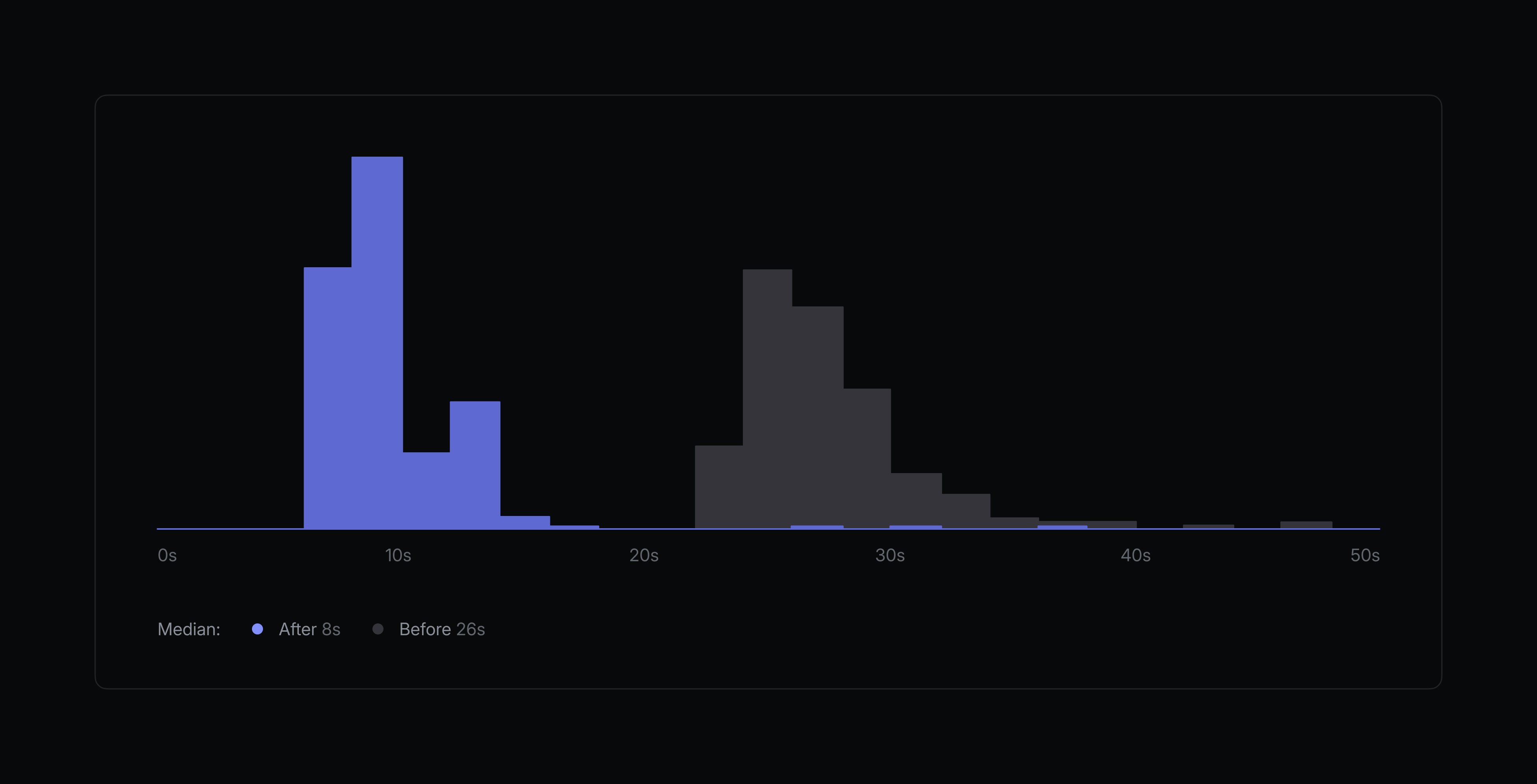
With the underlying infrastructure and individual checks running faster, we zoomed out to look at CI as a system. That drew our attention to the small jobs that sat in front of everything else. Every run starts by checking which paths a PR touched and whether these tests have already passed for the same inputs. We gate on those checks at the job level so skipped work never reserves a runner, but that also puts them directly on the critical path. None of the eight API test shards can start until they finish, making even small delays disproportionately important.

Fetch only what each job needs⁠

Several of our workflows start with a change-detection job that decides what runs next; for instance, it checks whether a diff contains a database migration and outputs a signal used to schedule the relevant database CI checks. These jobs were checking out the full working tree even though they needed only a small subset of it. We capped the fetch depth, which took the slowest of these gates from 94 seconds to 20, and removed checkout entirely from the jobs that never needed a working tree, reducing time spent on those from 27 seconds to 7. For commit push and merge-queue events, where we do have to diff paths, we found that a sparse, blobless checkout with limited history was enough, saving another 11 odd seconds.

Make checkout more resilient⁠

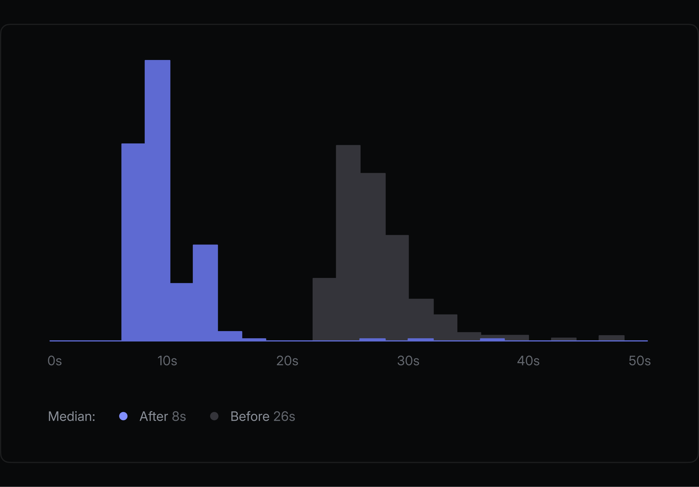
After we swapped the underlying runner infrastructure, we noticed that our checkout times (with actions/checkout) in our jobs had gotten longer and would sometimes hang. Because the third-party runners sit outside GitHub’s network, they rely on a direct IP link to reach GitHub. The provider traced the hangs to intermittent degradation on that link. Several of our workflows begin with a checkout, so a stalled fetch could delay the entire CI run.

To be resilient to the network instability, we replaced actions/checkout with a composite action of our own that retried with backoff, and sets GIT_HTTP_LOW_SPEED_LIMIT and GIT_HTTP_LOW_SPEED_TIME so a stalled connection aborts after about 30 seconds instead of hanging and also uses the checkout cache, which keeps a persistent git mirror on a sticky disk. The result was far fewer runs where a critical-path job sat idle waiting for checkout to finish.

Minimize what’s on the critical path⁠

Not every job on the critical path needed to be there. We were writing cache markers as part of the final check before merging, which meant a pull request could sit in the merge queue even after its tests had passed. We moved that write into a job that runs once the test shards finish but gates nothing, shaving 42 seconds from the merge path for every API pull request and merge-queue entry.

Together, these changes took roughly a minute off the required check for API pull requests on cache misses, while also reducing runner starts.

Reduce repeated setup⁠

From there, we turned to the setup cost repeated across every job, like booting a runner, installing packages, and provisioning build dependencies. That overhead means a job that does only seconds of useful work can end up consuming whole minutes of infrastructure time. Here are a few steps we took to work around that issue:

Preinstall shared dependencies in the CI image⁠

Our API test shards each spent 7 to 8 seconds installing the same Postgres client with apt on every run. We moved it into a small CI base image containing Node and the client, so each shard could start from an environment that was ready to run. We later added the required native build headers to the image after discovering that downloading them during setup could occasionally hang, shortening the tail.

Install only the dependencies each job needs⁠

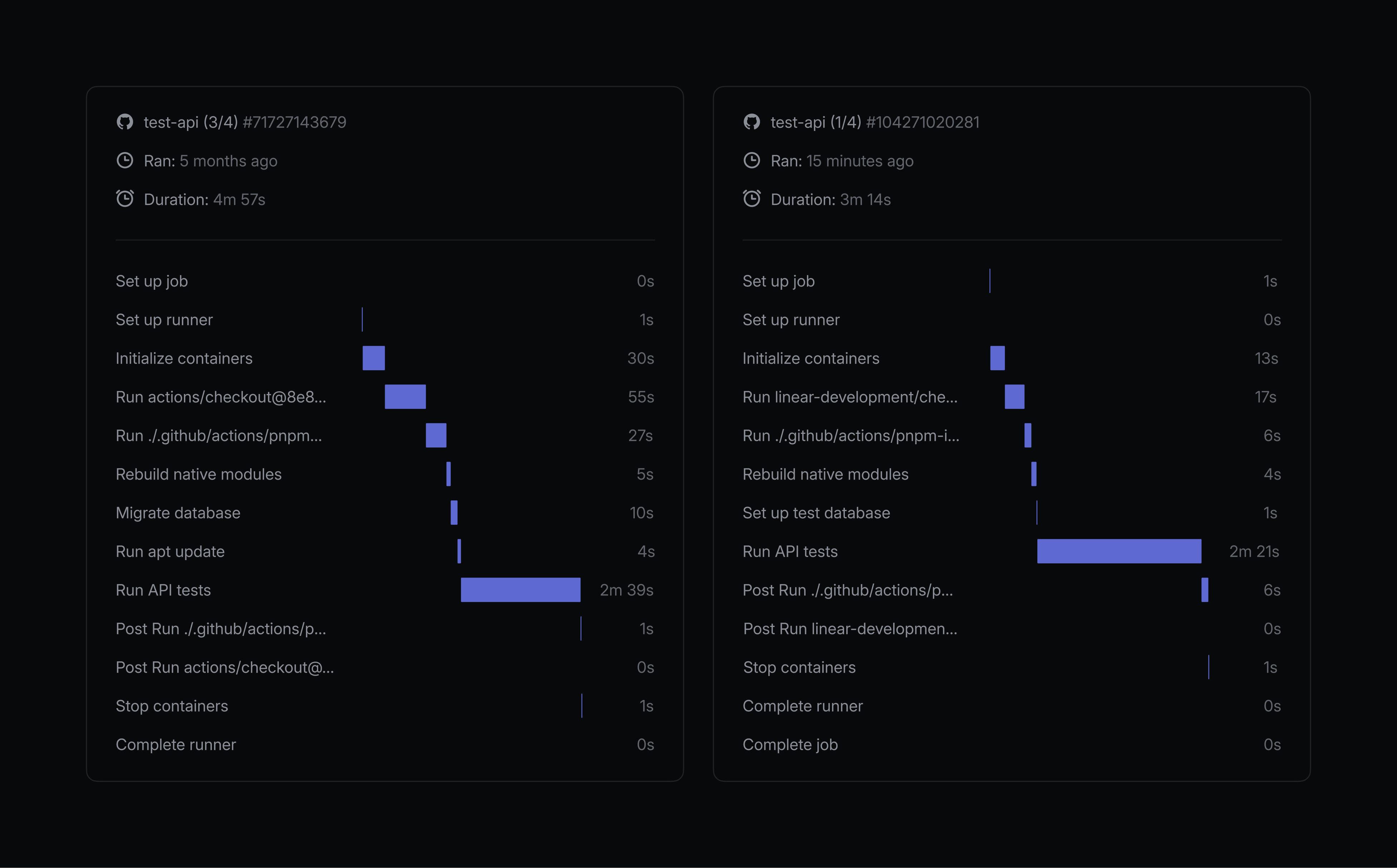
Linear’s codebase is a monorepo managed as a pnpm workspace. Our API test workflow was installing the entire workspace even though it only needed the API package and its dependencies. Restricting the install to our API package cut pnpm install from 44-73 seconds to 16-18 seconds. We applied the same pattern to API-adjacent jobs, which were each installing the full repository and uploading a dependency cache that later runs almost never hit.

Don’t cache when it’s faster to rebuild⁠

We also tested caching node_modules and found it was faster to rebuild. The cache key depended on a frequently changing lockfile, and even a cache hit took about 28 seconds to restore, compared with roughly 7.5 seconds for a filtered install. The cache was adding save time and variability without giving us any discernible advantage.

Together, these three changes reduced per-shard setup time by roughly 44%, from 110-140 seconds to 67-73 seconds.

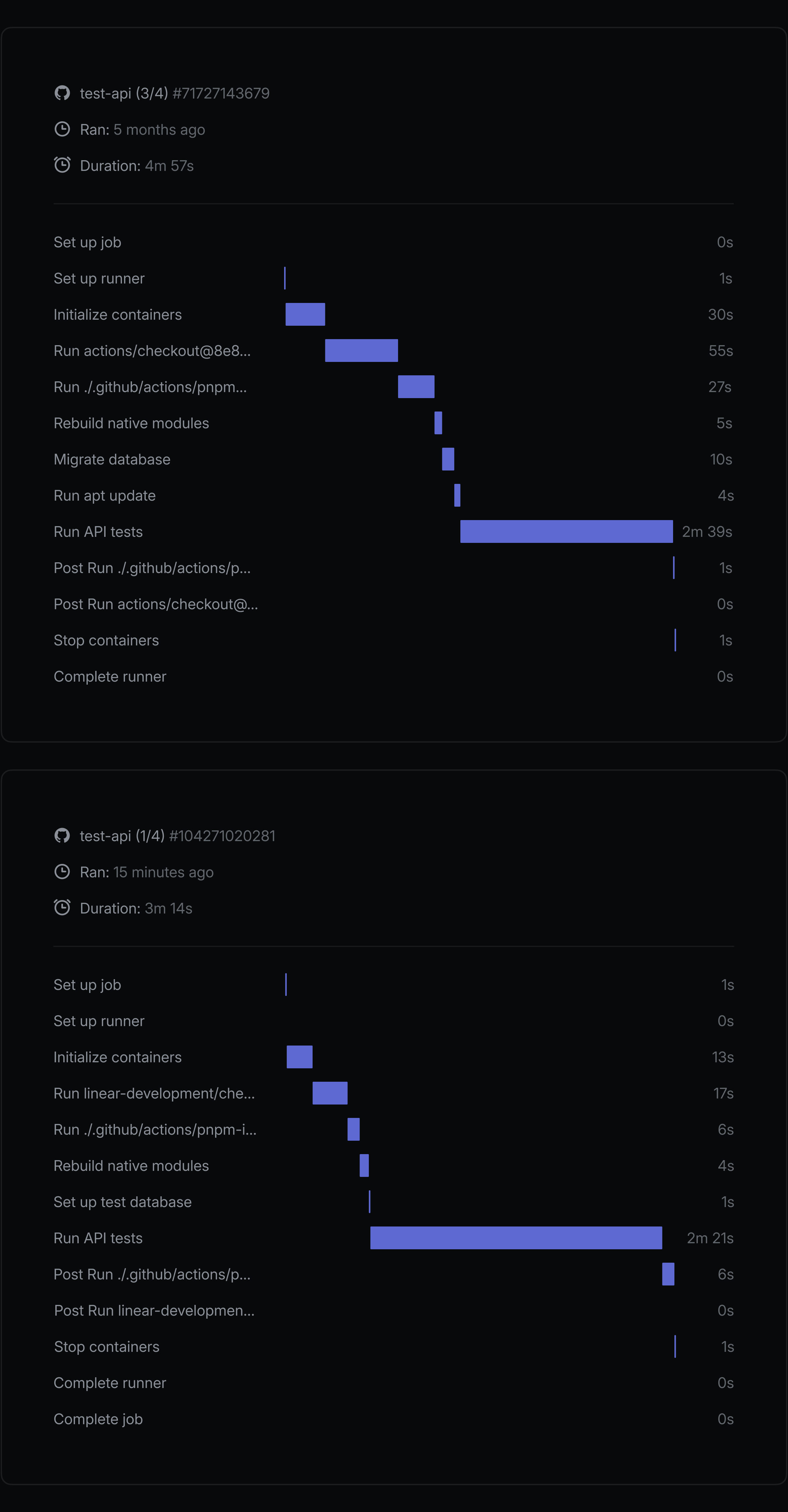
Beyond this, there were other forms of repeated setup we could avoid altogether.

Avoid replaying unchanged setup⁠

Some setup work only needs to be repeated when its inputs change. Our API containers, for example, were replaying the full database migration history on every run, even when a PR hadn’t changed the schema. For those cases, we switched to loading a generated schema snapshot and bootstrap file instead, cutting database setup from roughly 12 seconds to 1-2 seconds per container.

Batch short checks into fewer jobs⁠

Seven independent checks were each starting a runner, checking out the repository, and installing dependencies before doing only seconds of useful work. We consolidated them into two jobs, and then ran the seven tasks concurrently inside them. That reduced the number of times we paid the same setup overhead from seven to two. Based on June usage, the change saved roughly 87,000 runner-minutes per month, equivalent to 11.8% of our total CI usage.

Make test execution more efficient⁠

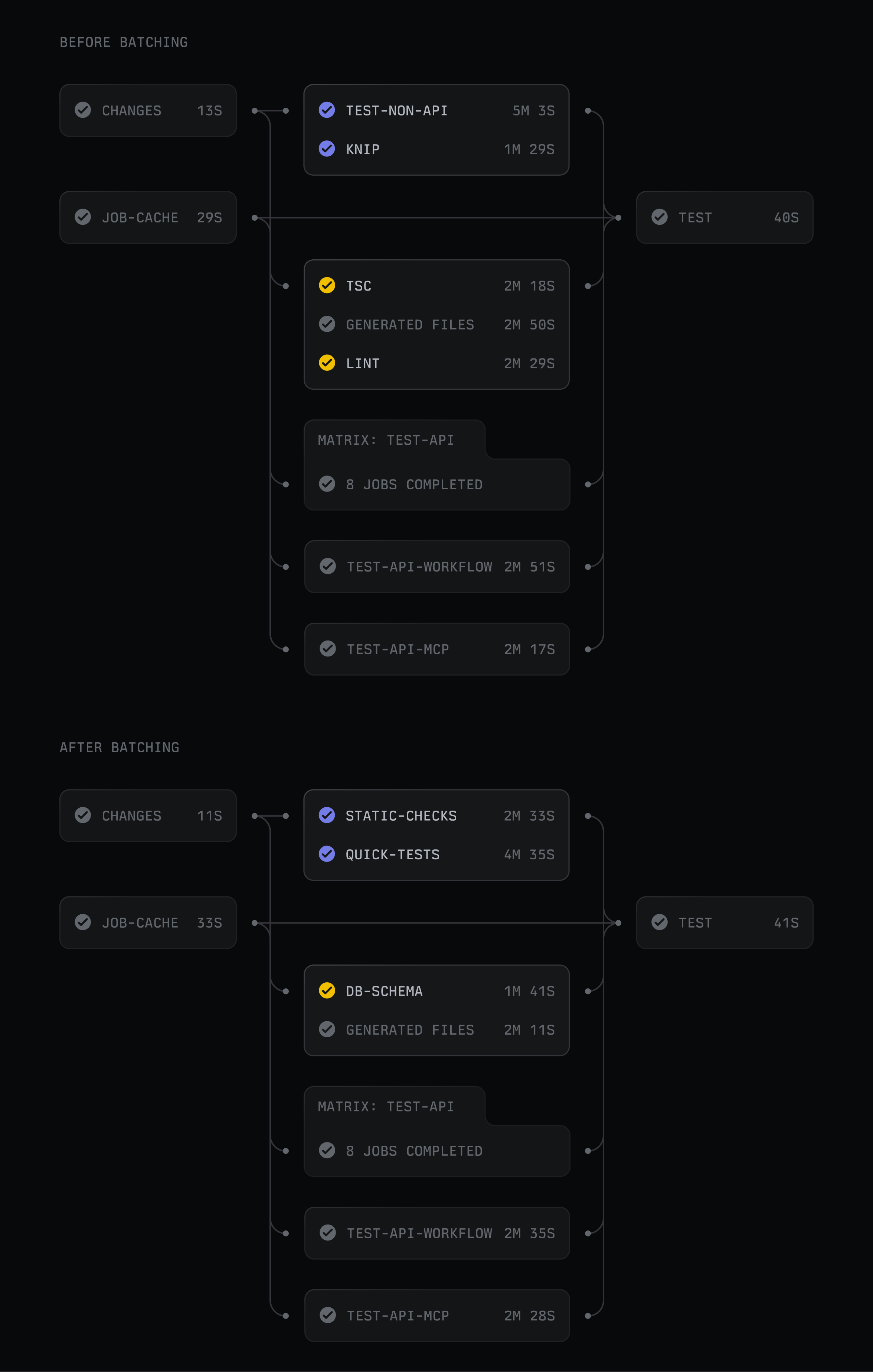
With the fixed cost of each test shard down, we could afford to parallelize the API suite more aggressively. It was the largest and one of the most frequently executed parts of our workflow, so improvements there had an outsized effect on merge time.

Balance work the way the test runner sees it⁠

Vitest, the test runner we use for our TypeScript test suites, distributes work by file rather than by the duration of individual tests. That meant a few unusually large test files could dominate a shard and effectively hold up completion of the entire suite, even when the other shards finished much earlier.

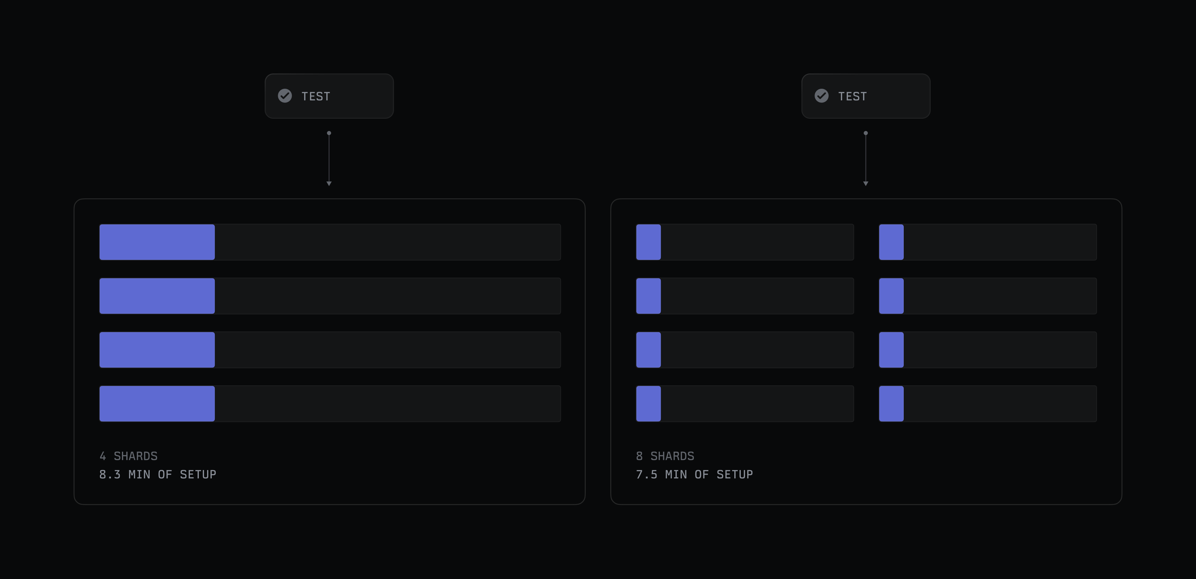
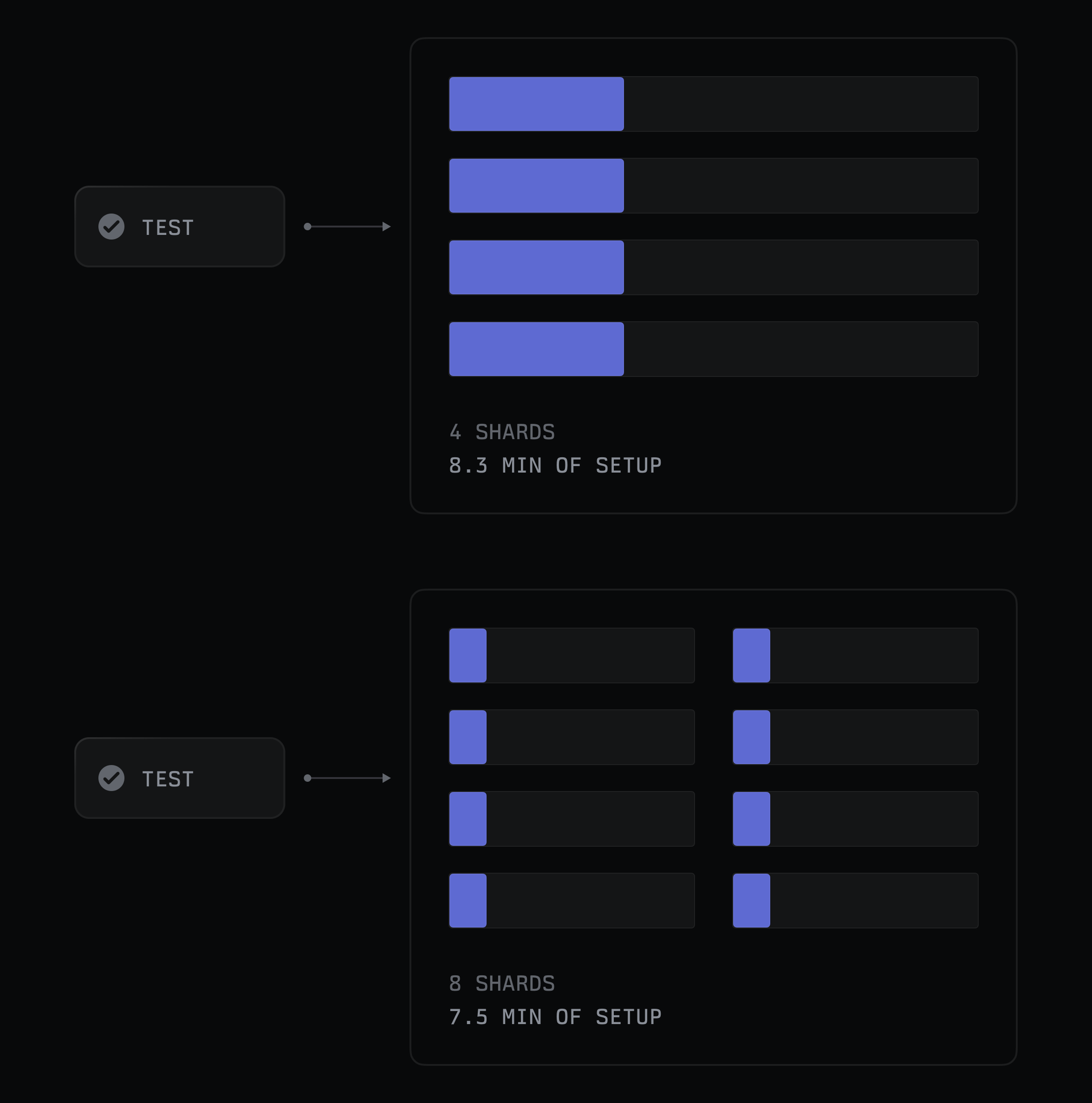
We split those large files into smaller, more focused files while preserving the structure of the tests, then evaluated different shard and runner configurations. We had already gone from three to four shards earlier in the year; moving to eight made the critical job roughly 19% faster and 19% cheaper in our initial benchmark. A week after the change, the slowest shard dropped from 5.25 minutes to 4.33 minutes.

Share module state only with strict isolation rules⁠

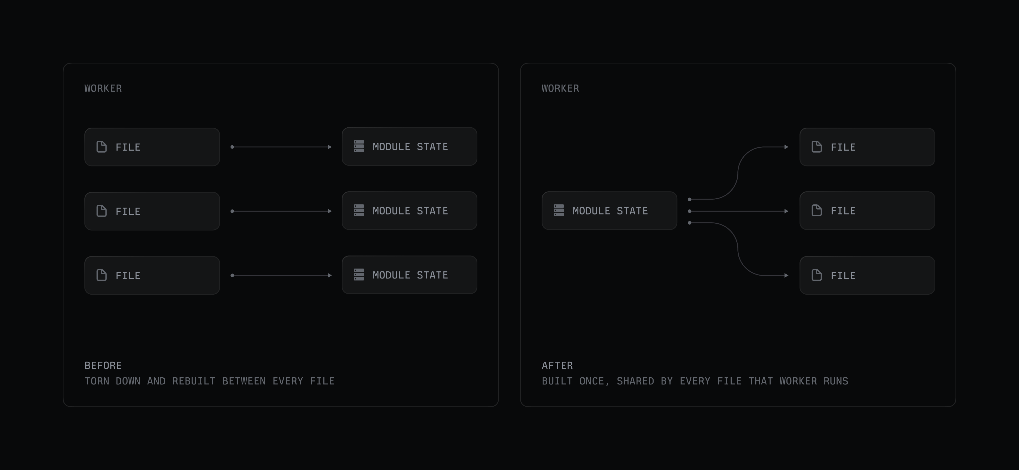
Vitest normally isolates every test file, which for us meant rebuilding the entity, GraphQL, and decorator graph in each test shard. We introduced an opt-in vitest project with isolate: false, allowing safe files to share a module registry within each worker.

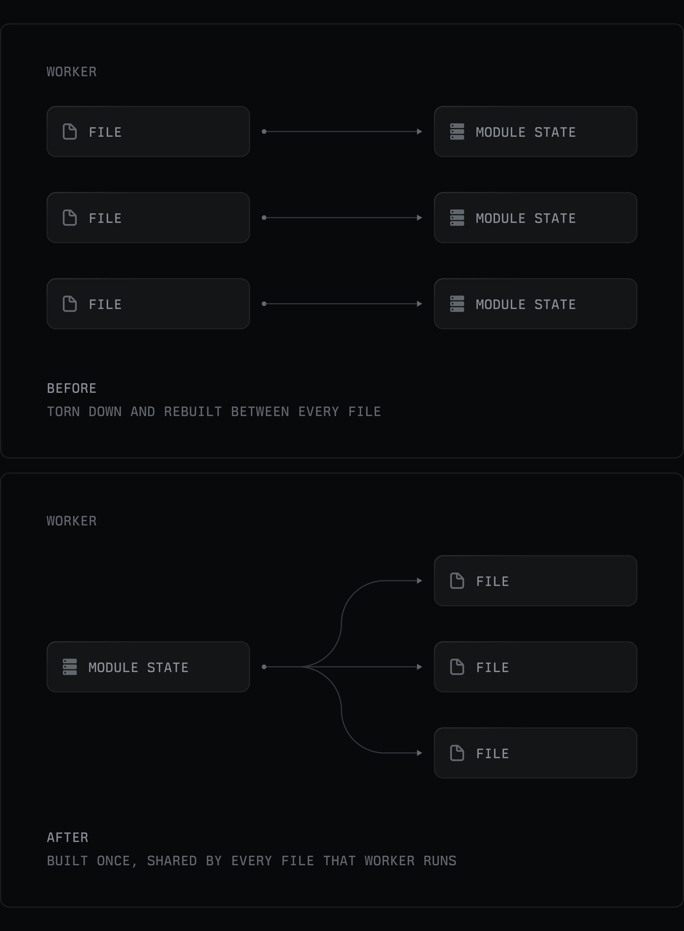
This was our largest single performance improvement, worth roughly 17% in monthly savings at our volume. The slowest shard fell from roughly 300-379 seconds to about 195 seconds, while total API-shard runner time dropped from about 32.8 to 22 minutes per run.

It was also the optimization with the highest correctness risk. We made eligibility explicit with an opt-in comment on every file, and added the necessary teardown for shared state. A handful of files used fake timers or shared state in ways we couldn’t untangle safely, so we left them in the isolated project. And because agents now write the majority of our tests, we updated our respective agent skills to account for this performance opt-in as well, so generated tests follow the same constraints by default.

Sharding is limited by setup overhead⁠

Further sharding only pays off when the fixed cost per shard is low, since doubling the shard count also doubles the workflow time spent on setup. The setup optimizations we referred to earlier are what made eight shards practical. At 110-140 seconds per shard, eight shards would have spent 15-19 minutes of runner time on setup alone, more than the tests themselves. Setup is now around 40 seconds, so eight shards spend less total setup time than four did before, while parallelizing the tests twice as far.

Improvements that compound across a system⁠

Had we not made a deliberate effort to improve CI earlier this year, today’s test suite would take roughly 11 minutes, close to double what developers wait now. And the work doesn’t end here. It’s clear that our codebase will continue to grow; we’re currently adding roughly 2,000 tests a week. Keeping CI fast as that happens will be a continued effort, much of it using what we learned through this process to new bottlenecks.

Mufeez Amjad

·September 21, 2026

Copy link

Source: Hacker News

The Tetris effect is one of psychology’s most easy to reproduce experiments.
Simply spend a bit of time playing the eponymous game every day for a few weeks.
After a little while, you’ll start recognizing familiar Tetromino shapes in clouds, buildings, and everyday objects.
You might even see them appear before your eyes when you start falling asleep.

Attention hijacking

There’s one lesson the Tetris effect teaches us: whatever you focus on long enough will end up shaping your thoughts.
This can be a good thing since it’s how we learn new skills and discover new ideas.
Sadly, less and less of our attention is focused intentionally.
Instead of picking what we want to see we let other people decide what is supposed to be good for us.

Do you want to watch a video?
YouTube knows you like cooking and art streams.
But why not also recommend a few clips about the stock market bubble, global warming, and the war in Iran.
Doomscrolling will make you stay longer and click on a few more ads.

Do you want to listen to music?
Just open a Spotify playlist and let the algorithm figure out what you like.
Please ignore the AI slop they will insert in between real songs to avoid paying royalties to real artists.

Do you want to know how your colleagues are doing?
Too bad, LinkedIn will bury any relevant career news between the opinion of complete strangers.
It is surely just a coincidence that those strangers happen to be shilling whatever Microsoft is invested in at the moment.

Do you want the opinion of strangers on a product?
Well those Redditors you wanted to ask are probably just a bunch of LLMs talking to a bunch of Russian trolls now.
I hope you didn’t value their opinion too much.

If, like me and most people, you spend the major part of your day focused on your device, there’s no doubt it’s affecting you.
And when you let someone else dictate what appears on your screen, it’s the same as giving them the key to your brain.

Back to an intentional internet

The internet wasn’t always like that.
Before recommendation algorithms were a thing, you had to decide what you would be doing on the computer.

You didn’t really have one big app that you could open and order it to entertain you.
Instead, you had a few dozen of bookmarks to websites, each with a specific idea in mind.
A site for video game news, that one website with lots of tutorials, a blog about anime that didn’t update often enough, a wiki about a TV show from the 90s…

Of course awful things existed on the web.
We had Encyclopedia Dramatica and Rotten.com, but you actually had to put the effort to go there if you wanted.
Nobody was going to put pictures of dead kids and far-right propaganda as a suggestion after a pancake recipe or a cat video.

The good thing is that this intentional internet is still around.
It has just been a bit buried below the corporate web, but it’s not very hard to find.
After all you’re on this blog, so you probably already have a good idea about it.

The main difference between this time and now is you.
When you want to get back to reading blogs, RSS feeds, and finish that tutorial instead of doomscrolling shorts, you have to get used to a slower internet.
One where content is not infinite and doesn’t get updated every click.

But like every habit, the only thing you have to do is to keep at it.
And if you pay enough attention to it, something will click in your brain.

Source: Hacker News

Source: Hacker News

We have the whole Oxide team coming to Emeryville this week for our
annual OxCon meetup. For a remote company, an in-person meeting is
uniquely energizing, and in preparation for that, we made some
t-shirts featuring Oxide logos that are an homage to past computer
companies.

Thanks to our designer
extraordinaire, Ben Leonard,
all of these homage shirts are amazing — but one of them was
simply too hot to leave as a surprise:

Unsurprisingly, this shirt has stirred up a bunch
of nostalgia for Sun. Much of the fondness for
Sun has been earned:
Oxide’s mission
comes directly from Scott McNealy’s epitaph for Sun — and Scott’s reflection that over 28 years he “never had to hide the newspaper in shame
from my children” remains
words that all companies should live by.

But the nostalgia can also become suffocating — to the point where folks
that post-date Sun may reasonably
demand to hear what Sun did wrong.
And of course, Sun did plenty wrong; while I was never ashamed to work for
Sun, I was not infrequently embarrassed by the stuff we screwed up.

Every Sun employee will have their own perspective on what Sun got wrong,
and
I talked about my own view in
a Hacker News comment in 2011.
I stand by that analysis, but another 15 years on (!), I would probably
distill things even further:
Sun had become bored with the mechanics of running a business.

Sun’s disinterest is embodied in an episode from 2005,
when a startup that was running its infrastructure on OpenSolaris
was looking to buy Sun gear.
This is — or should have been — a vindication of Sun
making Solaris open source: the startup was growing like a weed,
pioneering what we would later call cloud computing.
The startup was using Sun’s software, and wanted to buy a ton of
Sun hardware; the model worked!

Except, it didn’t. The customer could not get Sun to pick up the phone.
(And when Sun did pick up the phone, they tried to sell them the wrong
product.)
This was in sharp contrast to their experience with Dell: the startup filled out a web form in the
middle of the night, and the next morning…​

…​the phone rings, it’s Steve the local Dell account executive, and thus began the process where we all came under the impression that Steve actually worked for us. In less than 2 weeks we had some chances to “pitch” the company to get into a certain pricing tier, had all the servers in the datacenter, and had managed to get it all leased based purely on the company’s financials (no personal guarantees). And honestly, 95% of all of the work was done by Steve. I felt like a Big Company. I felt like Steve worked for me.

We know all of this because the startup did Sun the tremendous
service of writing it all up
in a blog entry,
The Sun Doesn’t Shine on Me.

I remember (vividly!) where I was when I read that blog entry:
we had just
started Fishworks,
and we were squatting in a corner of some abandoned Sun office
space while awaiting a more permanent home in San Francisco.
My heart sank as I read it, in part because it represented
so much strategic success, and yet was ultimately a story of operational
failure.
I remember thinking that a company that has become bored with
the mechanics of running a business cannot succeed — no matter how
successful its
strategy might otherwise be.

Sun continued for a few more years, and we tried like hell to
right the ship, but it wasn’t enough;
Sun didn’t make it.

As for me, after
I left Sun,
I would join that startup, the one upon whom the Sun did not shine.
And what happened to Steve from Dell? It turns out, the startup had the wisdom
to hire him too — and years later,
he and I started Oxide together.

For those outside of Sun, our homage to Sun (and to other defunct computer companies!) may seem purely nostalgic, but to us, it’s something deeper:
we admire these companies for the important things that they got
right, but we study them to learn what they got wrong. We honor
them best by learning from both — to be at once inspired and warned!

Source: Hacker News